ABSTRACT

We study the approximation of variational inequality related to American options problem. A simple proof to asymptotic behavior is also given using the theta time scheme combined with a finite element spatial approximation in uniform norm, which enables us to locate free boundary in practice.

Keywords:American Options, Finite Elements, Parabolic Variational Inequalities, Fixed Point, Asymptotic Behavior

1. Introduction

Since the work of Black-Scholes in 1973 see [1] , the financial markets have expanded considerably and traded products are increasingly numerous and sophisticated. Most widespread of these products are the options. The basic options are the options to sell and purchase, respectively called put and call. If option can be exercised at any time until maturity, we speak about American option otherwise it is a European option.

The two researchers provide a method of evaluation of European options by solving a partial derivative equation called (black-Scholes’s equation). However, we cannot get explicit formula for pricing of American options, even the most simple. The formalization of the problem of pricing American options as variational inequality, and its discretization by numerical methods, appeared only rather tardily in the article of Jaillet, Lamberton and Lapeyre see [2] . A little later, the book of Wilmott, Dewynne and Howison see [3] has made it much more accessible the pricing by L.C.P from American Option problem. For the problems at free boundary several numerical results have been obtained for parabolic and elliptic variational and quasi-variational inequality see [4] -[8] .

For our part, we are interested to asymptotic behavior of V.I related to the American options problem. Where we adapted to our problem result obtained in [4] and we eliminated an additional factor. We discretize the space by a space constructed from polynomials of degree 1 and the time by θ- scheme. Subsequently, we demonstrated the error estimate between the continuous solution and the discrete solution of the problem given by:

For, we have

and for, we have

We used the uniform norm, because it is a realistic norm, which gives us the approximation described above and which enables us to locate the free boundary, a crucial thing in practice of the American options.

The paper is organized as follows. In Section 2, we give the problem of American options as a parabolic variational inequality. In Section 3, we discretize by the finite elements method and we deal the stability of θ-scheme for our V.I. In Section 4, we adapt to our problem results obtained for similar problems see ([7] [9] ) namely a contraction associated with our problem which allows us to define an algorithm of Bensoussan-Lions [10] . Finally, in Section 5, we establish the estimate of the asymptotic behavior of θ-scheme by the uniform norm for American options problem.

2. Formulation of American Options Problem as Variational Inequality

In this section, we recall the context of our problem (see [11] -[13] ). An American option is a contract which gives the right to receive the payoff at some time, where. This payoff is then given as a function of the prices at the time t of n financial products constituting the underlying asset. Such as these prices are strictly positive, we set

(1)

and we express the payoff under the form

(2)

where

(3)

is a given regular function.

We assume that the following stochastic differential equation is satisfied by the logarithmic transformation of the prices

(4)

where is the interest rate, is invertible Volatility matrix and is a standard ndimensional Brownian motion defined on a probability space

The Continuous Problem

Under some assumptions on financial markets (no-arbitrage principle) see [2] [14] and the above assumptions one can prove, that is a solution of the following parabolic inequality:

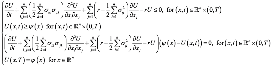(5)

Now we will give the variational inequality related to American options problem in a more compact form, where we starts by giving new notations and imposed certain conditions.

By a change of variable, the problem (5) becomes:

Find solution of

(6)

where K is a closed convex set defined as follows:

(7)

with

(8)

and is a bounded smooth domain in, with boundary.

A is an operator defined over by:

(9)

and the coefficients: where and are satisfy the following conditions:

(10)

(11)

(12)

f is a positive function.

For more detail on the parabolic inequality associated with American options problem (see [2] [13] [15] -[17] ).

We can reformulate the problem (6) to the following parabolic variational inequality:

(13)

where is a continuous bilinear form associated with operator A defined in (9). Namely,

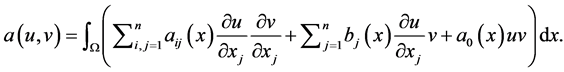(14)

Theorem 1 (Cf. [10] ): If, the problem (13) has an unique solution Moreover, one has

(15)

3. Study of the Discrete Problem

We decomposed into triangles and let denotes the set of all those elements, where is the mesh size. We assume that the family is regular and quasi uniform. Let denote the standard piecewise linear finite element space, and be the matrix with generic coefficients where, , are the basis function of the space, defined by where is a vertex of the considered triangulation.

We introduce the following discrete spaces of finite element constructed from polynomials of degree 1:

(16)

and

(17)

We consider r_h be the usual interpolation operator defined by:

(18)

The discrete maximum principle assumption (d.m.p): We assume that the matrix defined above is an M-matrix (Cf. [18] ).

Theorem 2 (Cf. [19] ): Let us assume that the bilinear form is weakly coercive in there exists two constants and such that

(19)

Notation:

3.1. Discretization

We discretize the space by a space discretization of finite dimensional constructed from polynomials of degree 1 and for the regularity of the solution see [20] . In a second step, we discretize the problem with respect to time using the θ-scheme. Therefore, we search a sequence of elements which approaches, with initial data

We apply the finite element method to approximate inequality (13), and the semi-discrete P.V.I takes the form of

(20)

Now, we apply the θ-scheme on the semi-discrete problem (20); for any and, we have for

(21)

where

(22)

(23)

We have that is admissible because

Thus we can rewrite (21) as: for and

(24)

Thus, our problem (24) is equivalent to the following coercive discrete elliptic variational inequality:

(25)

Such that

(26)

3.2. Stability Analysis of θ-Scheme for the P.V.I

The study of the stability of θ-scheme for the American options problem is adapted to [4] .

It is possible to analyze stabilitytaking advantage of the structure of eigenvalues of the bilinear form and wecall that W is compactly embedded in since is bounded.

Let the eigenvectors of form a complete orthonormal basis of in the finite dimensional problem. At each time step, can be expressed as well:

Moreover, let be the -orthogonal projection of into, that is, , one has

We are now in a position to prove the stability for, choosing in (21), thus we have for

(27)

For each, the inequalities (27) is equivalent to

(28)

Since are the eigenfunctions means

(29)

If one solves relative to, we find:

(30)

This inequality system stable if and only if

(31)

that is to say

(32)

means

(33)

So that this relation satisfied for all the eigenvalues of the bilinear form, we have to choose their highest value, we take it for

Lemma 1 (Cf. [4] ):

For the θ-scheme way is stable unconditionally i.e., stable

And if the θ-scheme is stable unless

(34)

With

(35)

(spectral radius of).

Notice that this condition is always satisfied if. Hence, taking the absolute value of (30), we have

(36)

also we deduce that

(37)

Remark 1 (Cf. [4] ):

We assume that the coerciveness assumption (19) is satisfied with, and for each, we find

(38)

where

4. Existence and Uniqueness for Discrete P.V.I

We consider that and are respectively the stationary solutions of the following continue and discrete inequalities:

(39)

(40)

where the bilinear form satisfies the coercivity condition.

Theorem 3 (Cf. [9] ): Under the previous assumptions, and the maximum principle, there exists a constant C independent of h such that

4.1. A Fixed Point Mapping Associated with Discrete Problem

We consider the mapping

(41)

where is the unique solution of the following discrete coercive V.I: find

Lemma 2 (Cf. [6] ): Under the d.m.p we have if then

Proposition 1: Under the previous hypotheses and notations, if we set, the mapping is a contraction in, i.e.,

(42)

Therefore, T_h admits a unique fixed point, which coincides with the solution of discrete coercive V.I (25).

Proof: For and, we consider (respectively, solution to discrete coercive variational inequality (25) with right-hand side (respectively).

Now, set

Since,

(because).

So using Lemma 2 gives

On the other hand, one has

Indeed, is solution of

thus

Therefore

Similarly, interchanging the roles of and we also get

Consequently,

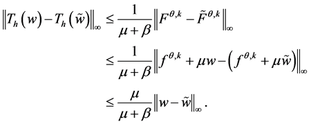
which is the desired result.

Remark 2: If we set, the mapping is a contraction in, i.e.,

(43)

Therefore, admits a unique fixed point, which coincides with the solution of discrete coercive V.I (25).

Proof: Under condition of stability, we have shown the θ-scheme is stable if and only if thus it can be easily show that

also it can be found that

which is the desired result.

4.2. Iterative Discrete Algorithm

We choose as the solution of the following discrete equation

(44)

where is a regular function given.

Now we give our following discrete algorithm

(45)

where is the solution of the problem (25).

Remark 3 cf. [7] : If we choose in (45) we get Bensoussan’s algorithm.

Proposition 2: Under the previous hypotheses and notations, we have the following estimate of convergence

(46)

And if

(47)

Proof: We set a first case, and we have

We assume that

so

thus

For a second case one can easily show that

which is the desired result.

5. Asymptotic Behavior

This section is devoted to the proof of principal result of the present paper, where we prove the theorem of the asymptotic behavior in -norm for parabolic variational inequalities.

Now, we evaluate the variation in between, the discrete solution calculated at the moment and, the continuous solution of (39).

Theorem 4: (The principal result). Under conditions of Theorem (3) and Proposition (2), we have for the first case

(48)

and for the second case

(49)

where C is a constant independent of h and k.

Proof: We have

thus

Then

Using the Theorem (3) and the Proposition (2), we have for

and for we have

6. Perspective

In the following, we will consolidate our theoretical results by numerical simulation, which allows us to locate the free boundary, a very interesting thing in practice to calculate the price of the American options.

Acknowledgements

The authors would like to thank the editor and referees for her/his careful reading and relevant remarks which permit them to improve the paper.

References

- Black, F. and Scholes, M. (1973) The Pricing of Options and Corporate Liabilities. Journal of Political Economy, 81, 637-654. http://dx.doi.org/10.1086/260062
- Jaillet, P., Lamberton, D. and Lapeyre, B. (1990) Variational Inequalities and the Pricing of American Options. Acta Applicandae Mathematicae, 213, 263-289. http://dx.doi.org/10.1007/BF00047211
- Wilmott, P., Dewyne, J. and Howison, S. (1993) Options Pricing: Mathematical Model and Computation. Oxford Financial Press.
- Boulaaras, S. and Haiour, M. (2011) L∞-Asymptotic Bhavior for a Finite Element Approximation in Parabolic QuasiVariational Inequalities Related to Impulse Control Problem. Applied Mathematics and Computation, 217, 6443-6450. http://dx.doi.org/10.1016/j.amc.2011.01.025
- Boulaaras, S. and Haiour, M. (2013) The Finite Element Approximation in Parabolic Quasi-Variational Inequalities Related to Impulse Control Problem with Mixed Boundary Conditions. Journal of Taibah University for Science, 7, 105-113. http://dx.doi.org/10.1016/j.jtusci.2013.05.005
- Boulbrachene, M. (2005) Pointwise Error Estimates for a Class of Elliptic Quasi-Variational Inequalities with Nonlinear Source Terms. Applied Mathematics and Computation, 161, 129-138. http://dx.doi.org/10.1016/j.amc.2003.12.015
- Boulbrachene, M. (2002) Optimal L∞-Error Estimate for Variational Inequalities with Nonlinear Source Terms. Applied Mathematics Letters, 15, 1013-1017. http://dx.doi.org/10.1016/S0893-9659(02)00078-2
- Lions, J.-L. and Stampacchia, G. (1967) Variational Inequalities. Communications on Pure and Applied Mathematics, 20, 493-519. http://dx.doi.org/10.1002/cpa.3160200302
- Cortey-Dumont, P. (1985) Sur les inéquations variationnelles a opérateurs non coercifs. Modélisation Mathématique et Analyse Numérique, 19, 195-212.
- Bensoussan, A. and Lions, J.-L. (1978) Applications des Inéquations Variationnelles en Controle Stochastique. Dunod, Paris, France.
- Karatzas, I. (1988) On the Pricing of American Options. Applied Mathematics & Optimization, 17, 37-60. http://dx.doi.org/10.1007/BF01448358
- Lamberton, D. and Villeneuve, S. (2003) Critical Price near Maturity for an American Option on a Dividend-Paying Stock. The Annals of Applied Probability, 13, 800-815. http://dx.doi.org/10.1214/aoap/1050689604
- Nystrom, K. (2008) On the Behaviour near Expiry for Multi-Dimensional American Options. Journal of Mathematical Analysis and Applications, 339, 644-654. http://dx.doi.org/10.1016/j.jmaa.2007.06.068
- Lamberton, D. and Lapeyre, B. (1991) Introduction au calcul stochastique applique a la finance. Ellipses.
- Achdou, Y. and Pironneau, O. (2005) Numerical Procedure for Calibration of Volatility with American Options. Applied Mathematical Finance, 12, 201-241. http://dx.doi.org/10.1080/1350486042000297252
- Oliver, P. (2004) Numerical Simulation of American Options. Thése Allemande.
- Trabelsi, F. (2011) Asymptotic Behavior of Random Maturity American Options. IAENG International Journal of Applied Mathematics, 41, 112-121.
- Ciarlet, P.G. and Raviart, P.A. (1973) Maximum Principle and Uniform Convergence for the Finite Element Method. Computer Methods in Applied Mechanics and Engineering, 2, 17-31. http://dx.doi.org/10.1016/0045-7825(73)90019-4
- Quarteroni, A. and Valli, A. (1994) Numerical Approximation of Partial Differential Equations. Springer, Berlin and Heidelberg.
- Blanchet, A., Dolbeault, J. and Monneau, R. (2005) Formulation de monotonie appliquées à des problèmes à frontiére libre et de modélisation en biologie. Thése de Doctorat, Université Paris Dauphine.