Applied Mathematics
Vol. 3 No. 12A (2012) , Article ID: 26083 , 14 pages DOI:10.4236/am.2012.312A296
Penalized Flexible Bayesian Quantile Regression
1Mathematical Science Department, School of Information Systems, Computing and Mathematics, Brunel University, Uxbridge, UK
2Statistics Department, College of Administration and Economics, Al-Qadisiyah University, Al Diwaniyah, Iraq
Email: *mapgaja@brunel.ac.uk
Received November 6, 2012; revised December 6, 2012; accepted December 13, 2012
Keywords: Adaptive Lasso; Lasso; Mixture of Gaussian Densities; Prior Distribution; Quantile Regression
ABSTRACT
The selection of predictors plays a crucial role in building a multiple regression model. Indeed, the choice of a suitable subset of predictors can help to improve prediction accuracy and interpretation. In this paper, we propose a flexible Bayesian Lasso and adaptive Lasso quantile regression by introducing a hierarchical model framework approach to enable exact inference and shrinkage of an unimportant coefficient to zero. The error distribution is assumed to be an infinite mixture of Gaussian densities. We have theoretically investigated and numerically compared our proposed methods with Flexible Bayesian quantile regression (FBQR), Lasso quantile regression (LQR) and quantile regression (QR) methods. Simulations and real data studies are conducted under different settings to assess the performance of the proposed methods. The proposed methods perform well in comparison to the other methods in terms of median mean squared error, mean and variance of the absolute correlation criterions. We believe that the proposed methods are useful practically.
1. Introduction
Quantile regression has become a widely used technique to describe the distribution of a response variable given a set of explanatory variables. It provides a more complete statistical analysis of the stochastic relationships among random variables. It has been applied in many different areas such as finance, microarrays, medical and agricultural studies—see Koenker [1] and Yu et al. [2] for more details.
Let  be a response variable and
  a
a  vector of covariates for the ith obsevation,
  is the ith row in the X matrix,
  is the inverse cumulative distribution function of
  given
given . Then, the relationship between
  and
and  can be modelled as
 , where
  is a vector of
  unknown parameters of interest and
 ![]() determines the quantile level.
determines the quantile level.
Koenker and Bassett [3] demonstrated that the regression coefficients  can be estimated by
 (1)
(1)
where  is the check function defined by
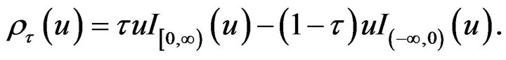 (2)
(2)
As a parametric possible link with minimizing the check function (1), Koenker and Machado [4] showed that maximum likelihood solution of the asymmetric Laplace (ASL) distribution is equivalent to the minimization of an objective function in (1). The idea of Koenker and Machado [4] was exploited by Yu and Moyeed [5] to propose Bayesian quantile regression. Yu and Moyeed [5] considered Markov Chain Monte Carlo (MCMC) methods for posterior inference. Recently, Bayesian approach for quantile regression has attracted much interest in literature. For example, Tsionas [6] developed Gibbs sampling algorithm for the quantile regression model, while Yu and Standard [7] proposed Bayesian Tobit quantile regression. Additionally, Geraci and Bottai [8] considered Bayesian quantile regression for longitudinal data using asymmetric Laplace distribution. Likewise, Kozumi and Kobayashi [9] and Reed and Yu [10] developed Gibbs sampling algorithms based on a location-scale mixture representation of the (ASL) distribution while Benoit and Poel [11] proposed Bayesian binary quantile regression.
Some researchers suggested nonparametric approaches to avoid the restrictive assumptions of the parametric approaches. See for example Walker and Mallick [12], Kottas and Gelfand [13], Hanson and Johnson [14], Hjort [15], Hjort and Petrone [16], Taddy and Kottas [17] and Kottas and Krnjajic [18]. Recently, Reich et al. [19] proposed a flexible Bayesian quantile regression model for independent and clustered data. The authors assumed that the error distribution is an infinite mixture of Gaussian densities. They called their method “flexible” because it does not impose a parametric assumptions (e.g., asymmetric Laplace) or shape restrictions on the residual distribution (e.g., mode at the quantile of interest) as with other approaches (personal communication with Reich).
The selection of predictors plays a crucial role in building a multiple regression model. The choice of a suitable subset of predictors can help to improve prediction accuracy. Also, in practice, the interpretation of a smaller subset of predictors is easier than a large set of predictors (Li et al. [20]). Variable selection by penalizing the classical least squares has attracted much research interest. See for example least absolute shrinkage and selection operator (Lasso) (Tibshirani [21]), smoothly clipped absolute deviation (SCAD) (Fan and Li [22]), Adaptive Lasso (Zou [23]) and the Bayesian approach of Park and Casella [24]. Although the classical least squares is popular for its mathematical beauty, it is not robust to outliers (Bradic et al. [25]; Koenker and Bassett [3]). For this reason, robust variable selection can be achieved using a rigorous method such as quantile regression.
The first use of regularization in quantile regression is made by Koenker [26]. The author put the Lasso penalty on the random effects in a mixed-effect quantile regression model to shrink individual effects towards a common value. Yuan and Yin [27] proposed Bayesian approach to shrink the random effects towards a common value by introducing ![]() penalty in the usual quantile regression check function. In addition, Wang et al. [28] proposed the LAD Lasso method which combines the idea of least absolute deviance (LAD) and Lasso for robust regression shrinkage and selection. Li and Zhu [29] developed the piecewise linear solution path of the
penalty in the usual quantile regression check function. In addition, Wang et al. [28] proposed the LAD Lasso method which combines the idea of least absolute deviance (LAD) and Lasso for robust regression shrinkage and selection. Li and Zhu [29] developed the piecewise linear solution path of the  penalized quantile regression. Moreover, Wu and Liu [30] considered penalized quantile regression with the SCAD and Adaptive Lasso penalties. Li et al. [20] suggested Bayesian regularized quantile regression. The authors proposed different penalties including Lasso, group Lasso and elastic net penalties. Alhamzawi et al. [31] extended the Bayesian Lasso quantile regression reported in Li et al. [20] by allowing different penalization parameters for different regression coefficients.
In this paper, we develop a flexible Bayesian framework for regularization in quantile regression model. Similar to Reich et al. [19], we assume the error distribution to be an infinite mixture of Gaussian densities. This work is quite different from Bayesian Lasso quantile regression employing asymmetric Laplace error distribution. In fact, the use of the asymmetric Laplace distribution is unattractive due to the lack of coherence (Kottas and Krnjajić [18]). For example, for different ![]() we have different distribution for the
we have different distribution for the ’s and it is difficult to reconcile these differences. Our motivating example is an analysis of body fat data which is previously analyzed by Johnson [32] and available in the package “mfp”. This study had a total body measurements of 252 men. The objective of this study is to investigate the relationship between the percentage body fat and 13 simple body measurements. In this paper we are interested in selecting the most significant simple body measurements for the quantile regression model, relating to the percentage body fat. Certain correlation is present between the predictors in the body fat data. For example, the correlation coefficient is 0.943 between the weight and the hip circumference, 0.916 between the chest circumference and the abdomen circumference, 0.894 between the hip circumference and the thigh circumference, 0.894 between the weight and the chest circumference, 0.887 between the weight and the abdomen circumference, 0.874 between the abdomen circumference and the hip circumference, and so on. The selection of variables is important in this application, in order to know which predictors have coefficients that vary among subjects. The high correlation between the predictors is an argument to use the Adaptive Lasso because the procedure deals with correlated predictors by using adaptive weights for the different predictors.
The remainder of this paper is organized as follows. A brief review of the flexible Bayesian quantile regression model for independent data is given in Section 2. Penalized flexible Bayesian quantile regression with Lasso and adaptive Lasso are proposed in Section 3 and Section 4, respectively. The experimental results are reported in Section 5. Finally, the conclusions are summarized in Section 6.
2. Flexible Bayesian Quantile Regression (FBQR)
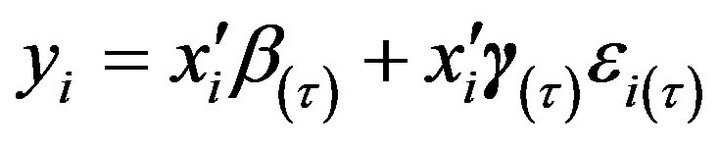
Following He [33], Reich et al. [19] considered the heteroskedastic linear regression model
 (3)
(3)
where  for all
  and the residuals
 ![]() are independent and identically distributed. The authors rewrote the above model as quantile regression model:
are independent and identically distributed. The authors rewrote the above model as quantile regression model:
 (4)
(4)
where  has τth quantile equal to zero,
  is the inverse cumulative distribution function of
![]() . To analyze
. To analyze ’s τth quantile,
  , the authors considered only distributions for the residual term with τth quantile equal to zero. Also, they fixed the element of
  corresponding to the intercept at 1 to separate out the scale of the errors from
 . For simplicity of notation, we will omit the subscript
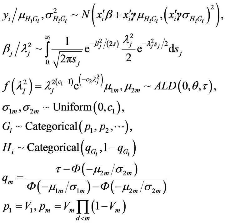
 ![]() in the remainder of the paper. From a Bayesian approach view, Reich et al. [19] assumed that the error term
in the remainder of the paper. From a Bayesian approach view, Reich et al. [19] assumed that the error term ![]() has a normal distribution with mean
has a normal distribution with mean  and variance
 , where
  and
and  are latent variables introduced to indicate the mixture component from which the ith observation is drawn. Under these assumptions, the conditional distribution of
  given
given  and
and  is given by:
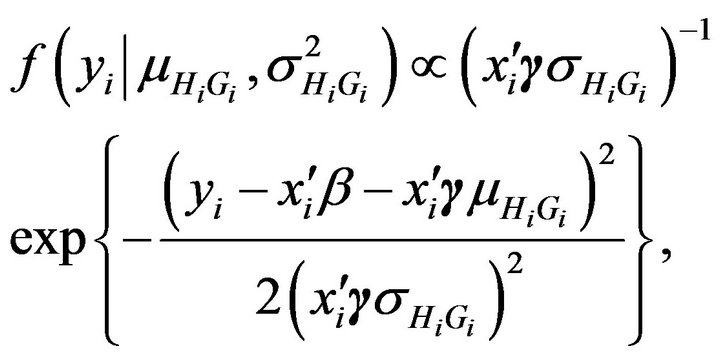 (5)
(5)
where  uniform
 and
and
 , where the parameters are the location, scale and the skewness. To specify a prior for
 , where the
  are the mixture proportions with
 , Reich et al. [19] defined the proportions
 through the latent variables
  which are independently identically distributed from beta
 where
where  controls the strength of the prior for
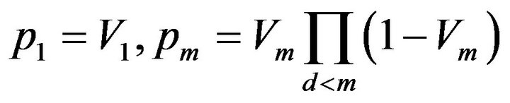
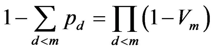
 . The first proportion is
  and the others are given by
 where
where .
.
The priors for the regression coefficients and scale parameters are  for large
  and
and
 . The prior for
  is vague normal prior subject to
  for all
  and the first element of
  corresponding to the intercept to be 1 to identify the scale of the residuals. As shown in Reich et al. [19], the performance of the above method is better than the frequentist method.
3. Flexible Bayesian Quantile Regression with Lasso Penalty (FBLQR)
Tibshirani [21] proposed the Lasso for simultaneous variable selection and parameter estimation. The Lasso, formulated in the penalized likelihood framework, minimizes the residual sum of squares with a constraint on the  norm of
 . The author stated the Lasso estimator can be interpreted as the posterior mode using normal likelihood and iid Laplace prior for
 . As extension to Lasso Tibshirani [21], Li and Zhu [29] suggested Lasso quantile regression for simultaneous estimation and variable selection in quantile regression models, and it is given by:
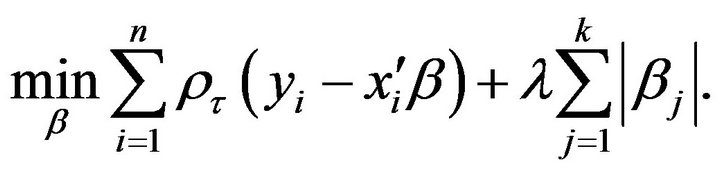 (6)
(6)
where  is the tuning parameter controlling the amount of penalty. The second term in (6) is the socalled
  penalty, which is essential for the success of the Lasso. In this paper we consider a fully Bayesian approach to enable exact inference and shrinkage of an unimportant coefficient to zero. We propose flexible Bayesian Lasso quantile regression which solves the following:
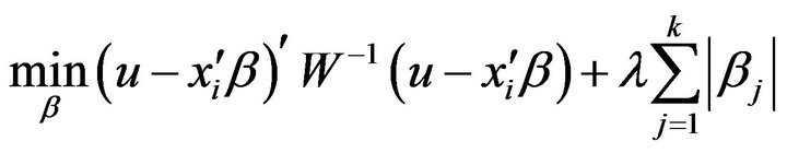 (7)
(7)
where  and W is a diagonal matrix with the element
  on the diagonal
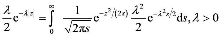
 . The second term of (7) can be represented as a mixture of normals (Andrews and Mallows [34])
 We further put gamma priors,
  , on the parameter
  (not
(not![]() ). Then, we have the following hierarchical model:
). Then, we have the following hierarchical model:
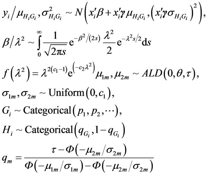
 where
where
 , the latent variables
  which are independently identically distributed from beta
 . The details of the Gibbs sampler are given in the appendix.
4. Flexible Bayesian Quantile Regression with Adaptive Lasso Penalty (FBALQR)
Fan and Li [22] studied a class of penalization methods including the Lasso. The authors showed that the Lasso can perform automatic variable selection because the  penalty is singular at the origin. On the other hand, the Lasso shrinkage produces biased estimates for the large coefficients, and thus it could be suboptimal in terms of estimation risk. Fan and Li [22] conjectured that the oracle properties do not hold for the Lasso. The Adaptive Lasso can be viewed as a generalization of the Lasso penalty. Basically the idea is to penalize the coefficients of different covariates at a different level by using adaptive weights. In the case of least squares regression, Zou [23] proposed the Adaptive Lasso in which adaptive weights are used to penalize different coefficients in the
  penalty. The author showed that the adaptive Lasso has the oracle properties that Lasso does not have. We propose Flexible Bayesian adaptive Lasso quantile regression which solves the following
 (8)
(8)
The second term of (8) can be represented as a mixture of normals (Andrews and Mallows [34])
 for each
 , we assume gamma prior,
 , on the parameter
 . Then we have the following hierarchical model:
where , the latent variables
which are independently identically distributed from beta .
.
5. The Experimental Results
5.1. A Simulation Study
A numerical study was conducted to assess the performance of the proposed methods. We generated  data-sets with size
  observations from
 , where
  are generated as independently and identically distributed standard normals. We simulated the error
 ![]() from three possible error distributions: standard normal, a
from three possible error distributions: standard normal, a  distribution with three degrees of freedom and Chi-squared distribution with three degrees of freedom
 . We use the following designs for the vector
 :
:
Design 1: 
Design 2: 
Design 3: 
Design 4: .
.
where the first element in  corresponding to the intercept.
Each simulated data set is analysis using five methods. We use our methods flexible Bayesian quantile regression with Lasso penalty (FBLQR) and flexible Bayesian quantile regression with Adaptive Lasso penalty (FBALQR) which are proposed in Sections 3 and 4 respectively. We compare the proposed methods with Lasso quantile regression (LQR) and the standard frequentist quantile regression (QR) using the “quantreg” package in R. Also, the proposed methods are compared with flexible Bayesian quantile regression (FBQR) (Reich et al. [19]).
The results of the simulation are presented in Tables 1-4 and Figures 1-4. From Tables 1-4 and Figures 1-4, according to the absolute correlation value of  and
and  and the median of the mean squared error (MMSE) for
 , it can be seen that the proposed methods (FBALQR and FBLQR) are better than the other three methods for all the distributions under consideration and for all the
 ![]() values. This indicates that the proposed methods give precise estimates even when the error distribution is an asymmetric. Most noticeably, when
values. This indicates that the proposed methods give precise estimates even when the error distribution is an asymmetric. Most noticeably, when  and
and  the FBALQR and FBLQR are more significantly efficient than the other methods. In addition, we can observe that the worst estimators for all the
 ![]() values are QR.
values are QR.
5.2. Body Fat Data
Percentage of body fat is one important measure of health, which can be accurately estimated by underwater weighing techniques. These techniques often require special equipment and are sometimes not easily achieved, thus fitting percentage body fat to simple body mea- surements is a convenient way to predict body fat. Johnson [32] introduced a data set in which percentage body fat and 13 simple body measurements (such as weight, height and abdomen circumference) are recorded for 252 men. The data set is available at the package (“mfp”). The response variable Y is the percent boday fat (%). The  predictor variables
 ![]() are, respectively, the age (years)
are, respectively, the age (years) , the weight (pounds)
 , the height (inches)
 , the neck circumference (cm)
 , the chest circumference (cm)
 , the abdomen circumference (cm)
 ,
,
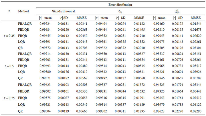
Table 1. Simulation results for FBALQR, FBLQR, FBQR, LQR and QR based on the linear model , design 1.
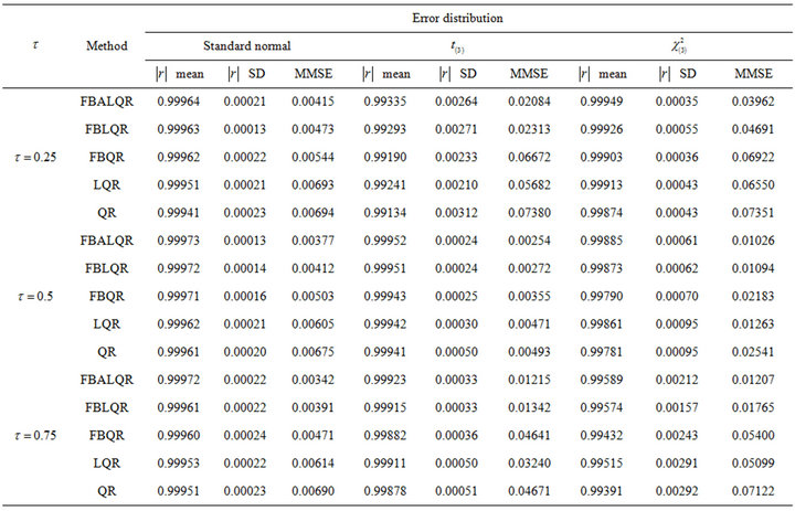
Table 2. Simulation results for FBALQR, FBLQR, FBQR, LQR and QR based on the linear model , design 2.
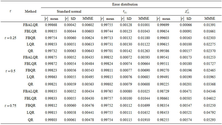
Table 3. Simulation results for FBALQR, FBLQR, FBQR, LQR and QR based on the linear model , design 3.
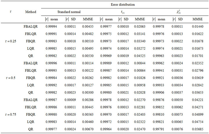
Table 4. Simulation results for FBALQR, FBLQR, FBQR, LQR and QR based on the linear model , design 4.
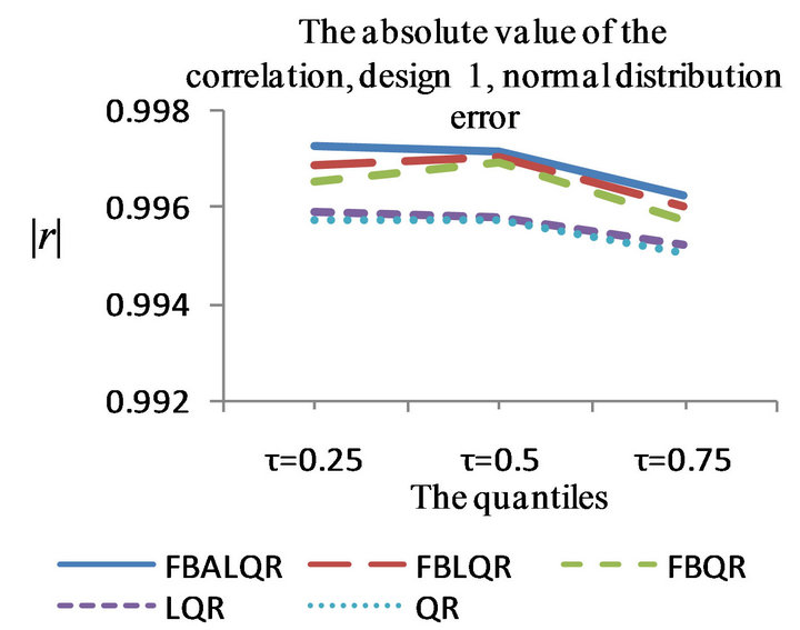
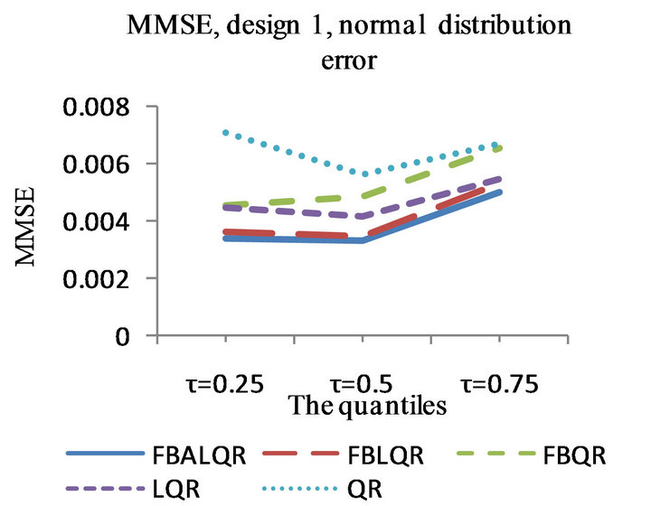
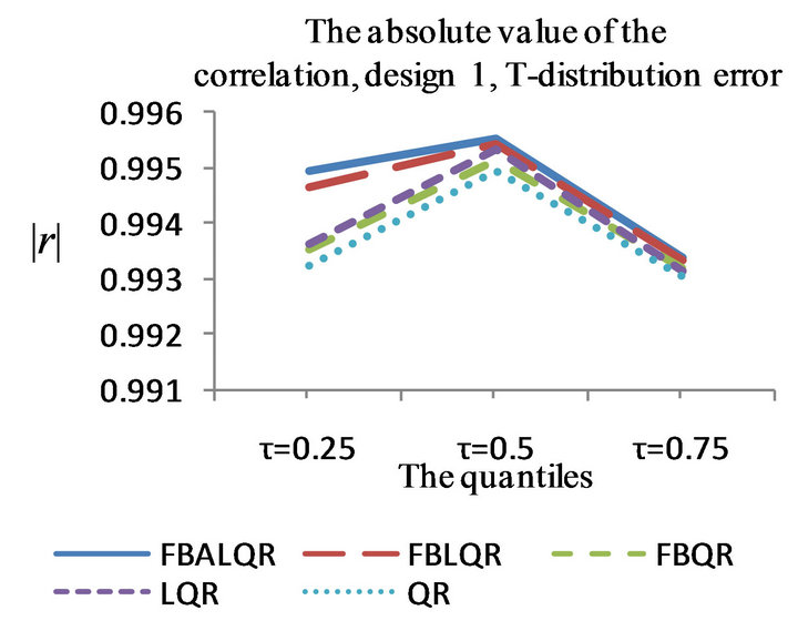
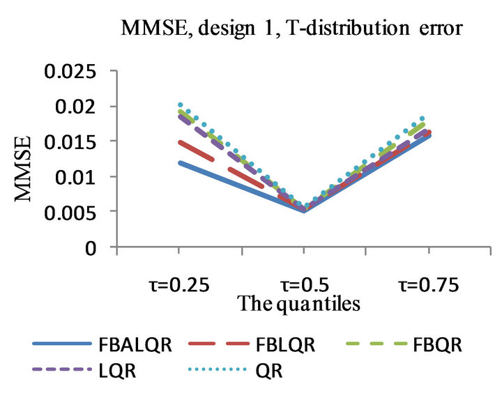
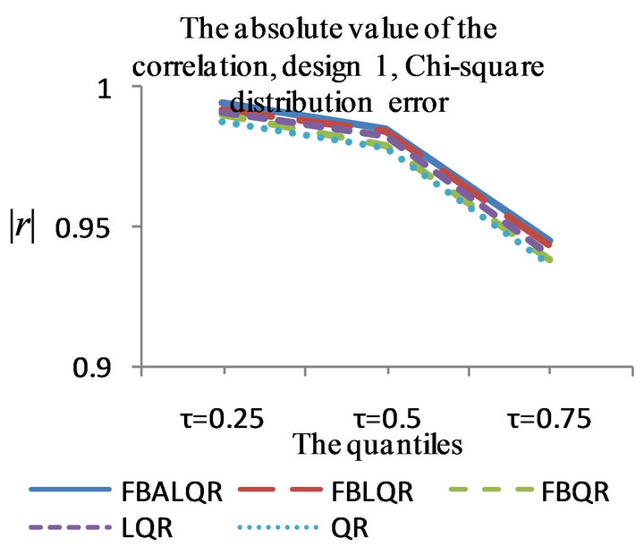
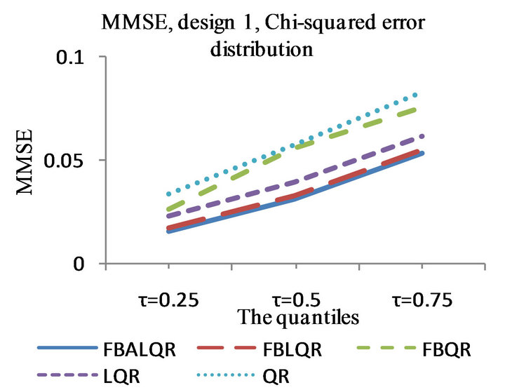
Figure 1. The left column explains the plots for the absolute value of the correlation between  and
and , design 1, and the error distributions are normal, T and Chi-square respectively. The right column explains the plots for the MMSE of
 , design 1, and the error distributions are normal, T and Chi-square respectively.
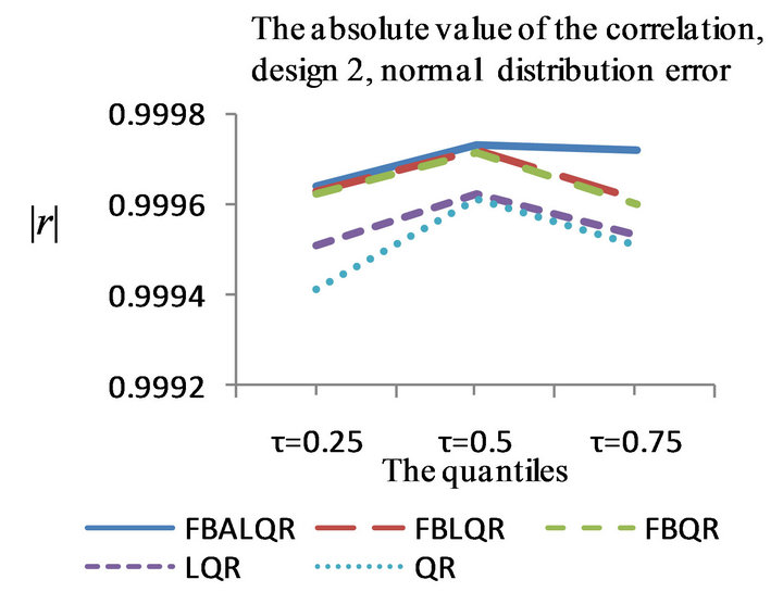
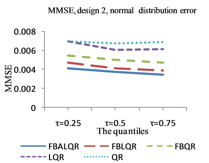
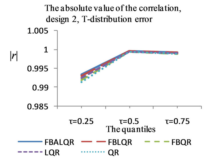

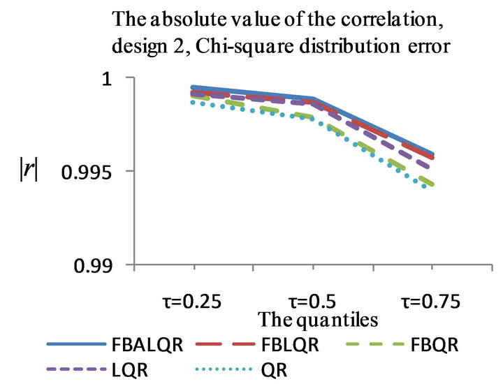

Figure 2. The left column explains the plots for the absolute value of the correlation between  and
and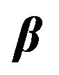 , model 2, and the error distributions are normal, T and Chi-square respectively. The right column explains the plots for the MMSE of
 , model 2, and the error distributions are normal, T and Chi-square respectively.
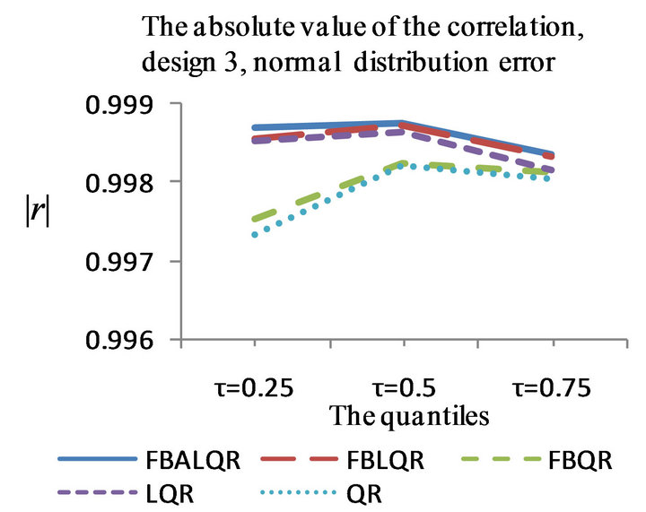
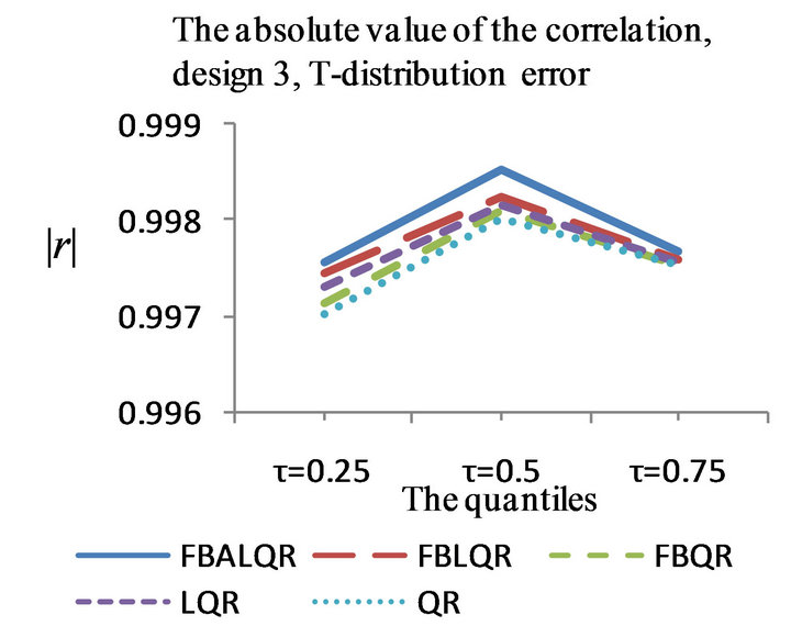
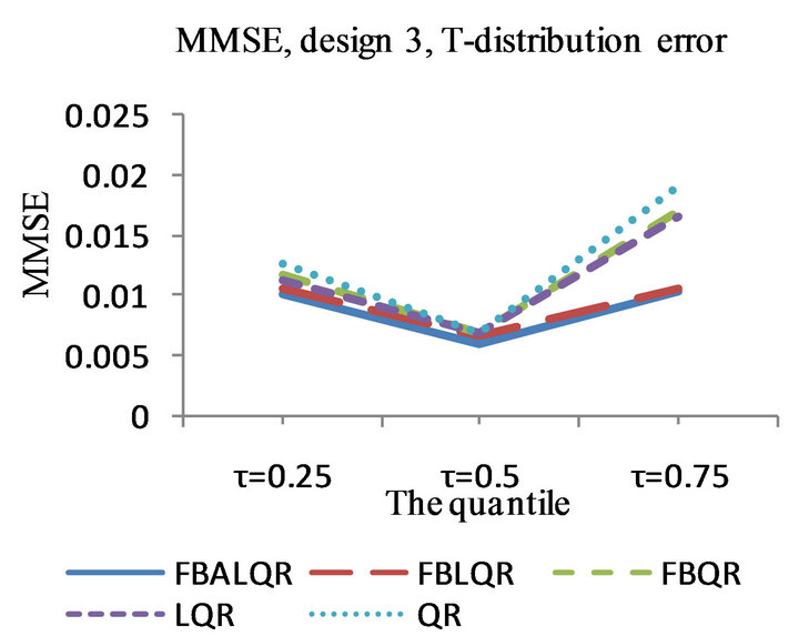
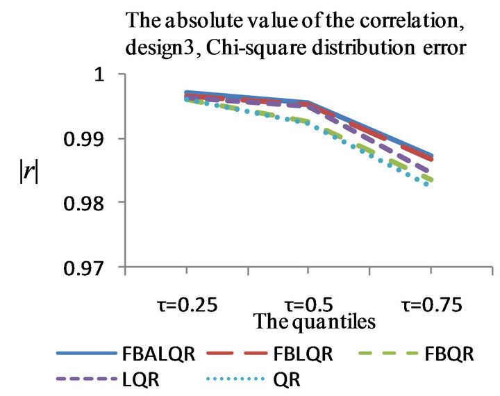
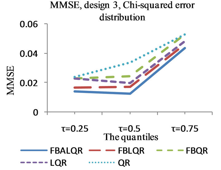
Figure 3. The left column explains the plots for the absolute value of the correlation between  and
and , model 3, and the error distributions are normal, T and Chi-square respectively. The right column explains the plots for the MMSE of
 , model 3, and the error distributions are normal, T and Chi-square respectively.
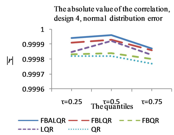
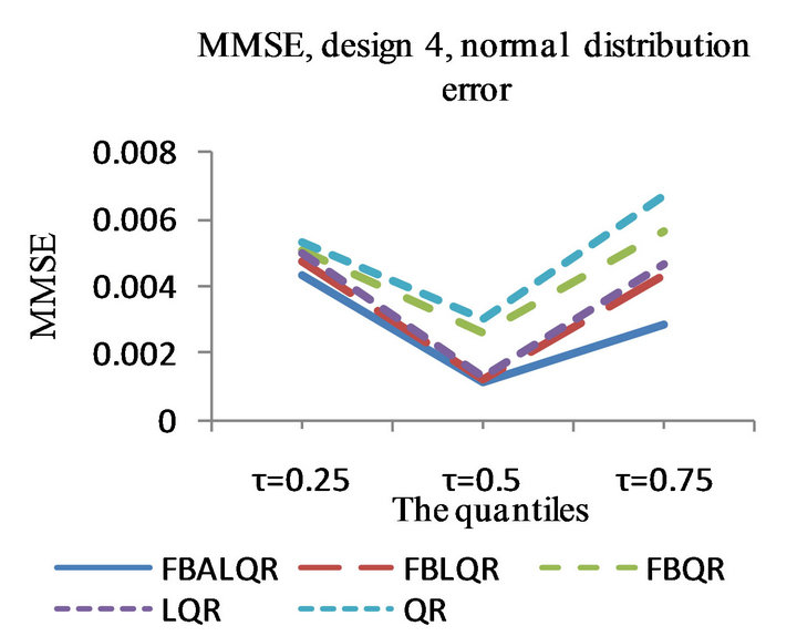
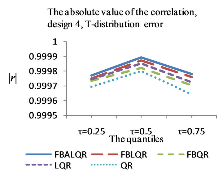
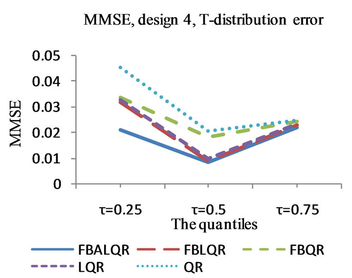
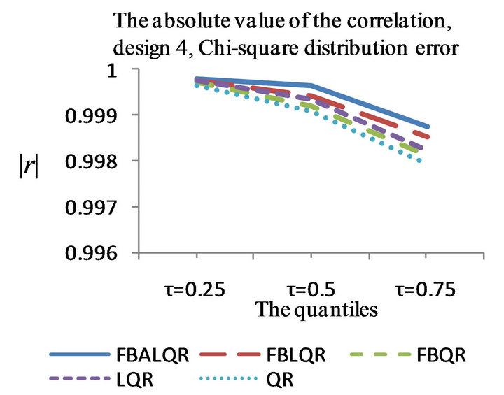
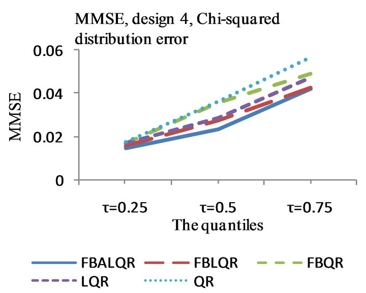
Figure 4. The left column explains the plots for the absolute value of the correlation between and
and , model 4, and the error distributions are normal, T and Chi-square respectively. The right column explains the plots for the MMSE of
 , model 4, and the error distributions are normal, T and Chi-square respectively.
The hip circumference (cm) , the thigh circumference (cm)
 , the knee circumference (cm)
 , the ankle circumference (cm)
 , the extended biceps circumference
 , the forearm circumference (cm)
  and the wrist circumference (cm)
 .
.
Hoeting et al. [35] and Leng et al. [36] analyzed this data set. Previous diagnostic checking (Hoeting et al. [35]; Leng et al. [36]) showed that it is reasonable to assume a linear regression model.
The results of the body fat data analysis are presented in Tables 5 and 6 and Figures 5 and 6. From Table 5 and Figure 5, we have the following observations. According to the mean squared error criterion, it can be seen that the performance of the proposed methods (FBALQR and FBLQR) is better than the performance of other methods. It is clear that the proposed methods give precise estimates. Again, we can see that when  and
and  the proposed methods are significantly more efficient than the other methods. The results of the simulation studies and real data example suggested that the proposed methods perform well.
6. Conclusion
In this study, we have proposed a flexible Bayesian Lasso and adaptive Lasso quantile regression by proposing a hierarchical model framework. We have theoretically investigated and numerically compared our proposed methods with the FBQR, Lasso quantile regression (LQR) and quantile regression (QR) methods. In order to
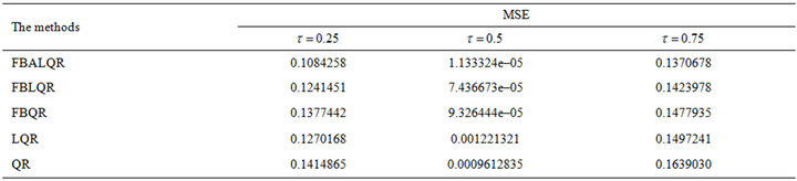
Table 5. MSE for  which is estimated by FBALQR, FBLQR, FBQR, LQR and QR based on body fat data for
 ,
,  and
and .
.
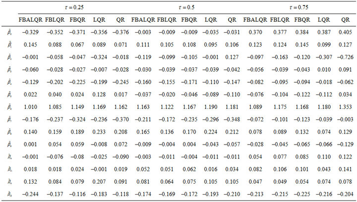
Table 6. The estimated  which is estimated by FBALQR, FBLQR, FBQR, LQR and QR based on body fat data for
  ,
, and
and .
.
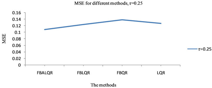
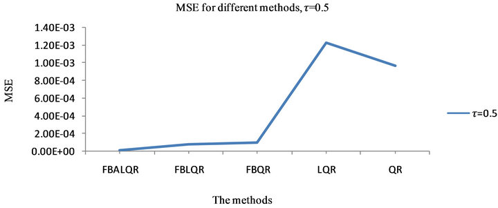
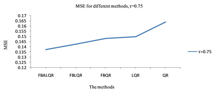
Figure 5. plots explain MSE for  which is estimated by FBALQR, FBLQR, FBQR, LQR and QR based on body fat data for
 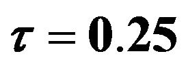 ,
, and
and .
.
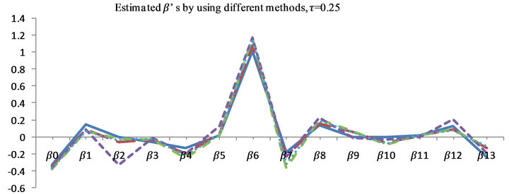
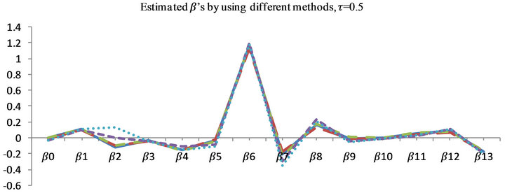
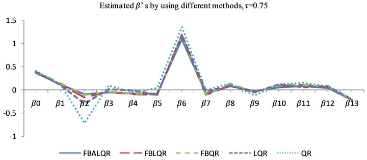
Figure 6. Plots explain the estimated  which is estimated by FBALQR, FBLQR, FBQR, LQR and QR based on body fat data for
 ,
,  and
and .
.
assess the numerical performance, we have conducted a simulation study based on the model  as described in Section 5 with error
 ![]() from three possible error distributions: standard normal, a
from three possible error distributions: standard normal, a  distribution with three degrees of freedom and Chi-squared distribution with three degrees of freedom
  and five designs for the vector β. From the simulation study and real data, we can conclude that the proposed methods perform well in comparison to the other methods and thus we believe that the proposed methods are practically useful.
REFERENCES
- R. Koenker, “Quantile Regression,” Cambridge University Press, Cambridge, 2005. doi:10.1017/CBO9780511754098
- K. Yu, Z. Lu and J. Stander, “Quantile Regression: Applications and Current Research Areas,” The Statistician, Vol. 52, No. 3, 2003, pp. 331-350. doi:10.1111/1467-9884.00363
- R. Koenker and G. Bassett Jr., “Regression Quantiles,” Econometrica, Vol. 46, No. 1, 1978, pp. 33-50. doi:10.2307/1913643
- R. Koenker and J. Machado, “Goodness of Fit and Related Inference Processes for Quantile Regression,” Journal of the American Statistical Association, Vol. 94, No. 448, 1999, pp. 1296-1310. doi:10.1080/01621459.1999.10473882
- K. Yu and R. A. Moyeed, “Bayesian Quantile Regression,” Statistics and Probability Letters, Vol. 54, No. 2, 2001, pp. 437-447. doi:10.1016/S0167-7152(01)00124-9
- E. Tsionas, “Bayesian Quantile Inference,” Journal of Statistical Computation and Simulation, Vol. 73, No. 9, 2003, pp. 659-674. doi:10.1080/0094965031000064463
- K. Yu and J. Stander, “Bayesian Analysis of a Tobit Quantile Regression Model,” Journal of Econometrics, Vol. 137, No. 1, 2007, pp. 260-276. doi:10.1016/j.jeconom.2005.10.002
- M. Geraci and M. Bottai, “Quantile Regression for Longitudinal Data Using the Asymmetric Laplace Distribution,” Biostatistics, Vol. 8, No. 1, 2007, pp. 140-154. doi:10.1093/biostatistics/kxj039
- H. Kozumi and G. Kobayashi, “Gibbs Sampling Methods for Bayesian Quantile Regression,” Technical Report, Kobe University, Kobe, 2009.
- C. Reed and K. Yu, “An Efficient Gibbs Sampler for Bayesian Quantile Regression,” Technical Report, Brunel University, Uxbridge, 2009.
- D. F. Benoit and D. Van den Poel, “Binary Quantile Regression: A Bayesian Approach Based on the Asymmetric Laplace Distribution,” Journal of Applied Econometrics, Vol. 27, No. 7, 2012, pp. 1174-1188. doi:10.1002/jae.1216
- S. Walker and B. Mallick, “A Bayesian Semi-Parametric Accelerated Failure Time Model,” Biometrics, Vol. 55, No. 2, 1999, pp. 477-483. doi:10.1111/j.0006-341X.1999.00477.x
- A. Kottas and A. Gelfand, “Bayesian Semi-Parametric Median Regression Modelling,” Journal of the American Statistical Association, Vol. 96, No. 465, 2001, pp. 1458- 1468. doi:10.1198/016214501753382363
- T. Hanson and W. O. Johnson, “Modeling Regression Error with a Mixture of Polya Trees,” Journal of the American Statistical Association, Vol. 97, No. 460, 2002, pp. 1020-1033. doi:10.1198/016214502388618843
- N. L. Hjort, “Topics in Nonparametric Bayesian Statistics,” In: P. J. Green, S. Richardson and N. L. Hjort, Eds., Highly Structured Stochastic Systems, Oxford University Press, Oxford, 2003, pp. 455-475.
- N. L. Hjort and S. Petrone, “Nonparametric Quantile Inference Using Dirichlet Processes,” In: V. Nair, Ed., Advances in Statistical Modeling and Inference: Essays in Honor of Kjell A. Doksum, World Scientific, Singapore City, 2007, pp. 463-492. doi:10.1142/9789812708298_0023
- M. Taddy and A. Kottas, “A Nonparametric Model-Based Approach to Inference for Quantile Regression,” Technical Report, UCSC Department of Applied Math and Statistics, 2007.
- A. Kottas and C. M. Krnjajić, “Bayesian Nonparametric Modelling in Quantile Regression,” Scandinavian Journal of Statistics, Vol. 36, No. 3, 2009, pp. 297-319.
- B. Reich, H. Bondell and H. Wang, “Flexible Bayesian Quantile Regression for Independent and Clustered Data,” Biostatistics, Vol. 11, No. 2, 2010, pp. 337-352. doi:10.1093/biostatistics/kxp049
- Q. Li, R. Xi and N. Lin, “Bayesian Regularized Quantile Regression,” Bayesian Analysis, Vol. 5, No. 3, 2010, pp. 1-24. doi:10.1214/10-BA521
- R. Tibshirani, “Regression Shrinkage and Selection via the Lasso,” Journal of the Royal Statistical Society Series B, Vol. 58, No. 1, 1996, pp. 267-288.
- J. Fan and R. Li, “Variable Selection via Nonconcave Penalized Likelihood and Its Oracle Properties,” Journal of the American Statistical Association, Vol. 96, No. 456, 2001, pp. 1348-1360. doi:10.1198/016214501753382273
- H. Zou, “The Adaptive Lasso and Its Oracle Properties,” Journal of the American Statistical Association, Vol. 101, No. 476, 2006, pp. 1418-1429. doi:10.1198/016214506000000735
- T. Park and G. Casella, “The Bayesian Lasso,” Journal of the American Statistical Association, Vol. 103, No. 482, 2008, pp. 681-686. doi:10.1198/016214508000000337
- J. Bradic, J. Fan and W. Wang, “Penalized Composite Quasi-Likelihood for Ultrahigh-Dimensional Variable Selection,” Journal of Royal Statistics Society Series B, Vol. 73, No. 3, 2010, pp. 325-349. doi:10.1111/j.1467-9868.2010.00764.x
- R. Koenker, “Quantile Regression for Longitudinal Data,” Journal of Multivariate Analysis, Vol. 91, No. 1, 2004, pp. 74-89. doi:10.1016/j.jmva.2004.05.006
- Y. Yuan and G. Yin, “Bayesian Quantile Regression for Longitudinal Studies with Non-Ignorable Missing Data,” Biometrics, Vol. 66, No. 1, 2010, pp. 105-114. doi:10.1111/j.1541-0420.2009.01269.x
- H. Wang, G. Li and G. Jiang, “Robust Regression Shrinkage and Consistent Variable Selection through the LAD,” Journal of Business and Economic Statistics, Vol. 25, No. 3, 2007, pp. 347-355. doi:10.1198/073500106000000251
- Y. Li and J. Zhu, “L1-Norm Quantile Regressions,” Journal of Computational and Graphical Statistics, Vol. 17, No. 1, 2008, pp. 1-23.
- Y. Wu and Y. Liu, “Variable Selection in Quantile Regression,” Statistica Sinica, Vol. 19, No. 2, 2009, pp. 801- 817.
- R. Alhamzawi, K. Yu and D. Benoit, “Bayesian Adaptive Lasso Quantile Regression,” Statistical Modelling, Vol. 12, No. 3, 2012, pp. 279-297. doi:10.1177/1471082X1101200304
- R. W. Johnson, “Fitting Percentage of Body Fat to Simple Body Measurements,” Journal of Statistics Education, Vol. 4, No. 1, 1996, pp. 236-237.
- X. He, “Quantile Curves without Crossing,” The American Statistician, Vol. 51, No. 2, 1997, pp. 186-192. doi:10.1080/00031305.1997.10473959
- D. F. Andrews and C. L. Mallows, “Scale Mixtures of Normal Distributions,” Journal of Royal Statistics Society Series B, Vol. 36, No. 1, 1974, pp. 99-102.
- J. A. Hoeting, D. Madigan, A. E. Raftery and C. T. Volinsky, “Bayesian Model Averaging: A Tutorial,” Statistical Science, Vol. 14, No. 4, 1999, pp. 382-417.
- C. Leng, M. N. Tran and D. Nott, “Bayesian Adaptive Lasso,” Technical Report, 2010. http://arxiv.org/PScache/arxiv/pdf/1009/1009.2300v1.pdf
Appendix
The details of Gibbs sampler for the penalized flexible Bayesian Lasso quantile regression are given as follows:
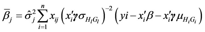
1) The full conditional distribution of  is multivariate normal distribution
 where
where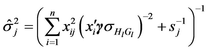 , and
, and
 .
.
2) The full conditional distribution of  is inverse Gaussian
  where
where  and
and
 .
.
3) The full conditional distribution of  is
is
Given  and
and , the parameters
  and the standard deviation parameters can be updated using Gaussian distribution. The group indicators
  are also updated using Metropolis-Hasting sampling (see Reich et al. [19] for more details). The full conditional distribution for all parameters in the penalized flexible Bayesian Adaptive Lasso quantile regression is similar to the above description except for the full conditional distributions for
  and
and  which are given by 1) The full conditional distribution of
  is inverse Gaussian
  where
where
 and
and .
.
2) The full conditional distribution of  is
is
 .
.
NOTES
*Corresponding author.