Applied Mathematics
Vol. 3 No. 6 (2012) , Article ID: 20356 , 7 pages DOI:10.4236/am.2012.36095
Asymptotic Comparison of Method of Moments Estimators and Maximum Likelihood Estimators of Parameters in Zero-Inflated Poisson Model
1Department of Statistics, Bangalore University, Bangalore, India
2Maharani’s Science College for Women, Bangalore, India
Email: nanzundan@gmail.com, raviisec@yahoo.co.uk
Received December 16, 2011; revised April 28, 2012; accepted May 6, 2012
Keywords: Zero-Inflated Poisson Model; Maximum Likelihood and Moment Estimators; EM Algorithm; Asymptotic Relative Efficiency
ABSTRACT
This paper discusses the estimation of parameters in the zero-inflated Poisson (ZIP) model by the method of moments. The method of moments estimators (MMEs) are analytically compared with the maximum likelihood estimators (MLEs). The results of a modest simulation study are presented.
1. Introduction
Zero-inflated models have found applications in situations where excess number of zero observations are generated. The application of the zero-inflated Poisson model by Lambert [1] in a count regression model is well known. Recently Couturier et al. [2] have used the zeroinflated truncated generalized Pareto distribution for the analysis of radio audience data.
The ZIP model is introduced in this section in the context of a practical situation. Maximum likelihood estimation of the parameters involved in the model is discussed in Section 2. The MMEs of the parameters are obtained in Section 3. The ZIP model is shown to be a member of the two-parameter exponential family and hence the asymptotic normality of the MMEs is established. Further, in Section 4, the details of computing the Fisher information matrix corresponding to this model are shown. In Section 5, the MMEs and the MLEs are asymptotically compared. Also, an empirical evidence for the asymptotic result is given through a modest simulation study in Section 6.
A random variable X is said to have a zero-inflated Poisson distribution, if its probability mass function (p.m.f.) is given by
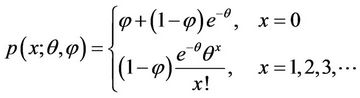 (1.1)
(1.1)
with ,
, . Note that
where 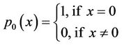 and
and 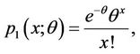
Thus the distribution of X is a convex combination of a distribution degenerate at zero and a Poisson distribution with mean θ. This is known as the zero-inflated Poisson model.
2. Maximum Likelihood Estimation
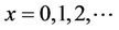
Let X = (X1, X2, X3, ∙∙∙, Xn) be a random sample on X with the p.m.f. specified in (1.1). Then the likelihood function is given by
 (2.1)
(2.1)
where 
It is obvious that the above likelihood function does not yield closed form expressions for the MLEs of θ and .
.
Yip [3] has shown that the conditional MLE of θ treating  as a nuisance parameter, is the solution of
 (2.2)
(2.2)
where and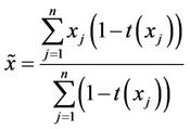 . The conditional MLE of θ also has no closed form expression and it has to be computed using a numerical procedure. Of course, it is much easier than computing the MLE of θ by maximizing (2.1). He has also observed that finding the values of θ and
  that maximize the likelihood function (2.1) is difficult because of its flat surface and boundary problem. Also, it is not necessary that the global maximum is located for every observed sample (See [3]). Kale [4] has obtained the optimal estimating equation for θ treating
  as a nuisance parameter when
  is the p.m.f. of a general power series distribution. When
  is the p.m.f. of a Poisson distribution with mean θ, the optimal estimating equation obtained by Kale [4] for θ reduces to (2.2).
Estimating  may be of significant interest and it cannot be treated as a nuisance parameter.
EM Algorithm
When the likelihood function has a complicated structure and maximizing it by numerical methods is difficult, a simple alternative procedure is the EM-algorithm developed by Dempster et al. [5]. Nanjundan [6] has computed the MLEs of θ and  using the EM algorithm. He has obtained the Eand M-steps by rewriting the likelihood function so as to accommodate missing data.
Let
 .
.
Then, we have
 . Suppose that
  is the observed sample on X. Then
 becomes the complete sample when
  is augmented with
 . If
. If , then
  and If
 , then and
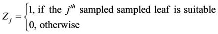
  or 1. In other words,
  , we have no information on
  Hence
Hence  can be treated as the missing data.
The likelihood function of the complete data is given by
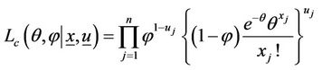
where 
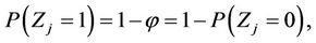
In the E-step, the expectation of the likelihood function of the complete data is taken and E(Z) is replaced by the conditional expectation  where
where  and
and  are respectively the initial estimates θ and
  In the M-step
  is maximized with respect to θ and
  If
If  and
and  are the values of θ and
  which maximize
 , then the E-step is repeated using
  and
and .
.
The computational details of these steps can be summarized as follows.
1) Choose the initial estimates of  and
and  by
by
 and
and 
where  and ng = number of
  and n0 = number of
  equal to zero.
2) Compute .
.
3) Using the realization (x1, x2, ∙∙∙, xn) of the observed sample, compute the improved estimates of θ and  by
by
4) Repeat steps 2) and 3) until the difference between the successive  [or
[or ] values is less than a desired threshold value.
The corresponding values of  and
and  are the MLEs of θ and
  respectively (See [5]). Unlike Fisher’s method of scoring, the EM algorithm does not yield the estimate of the standard errors of the MLEs as a by product.
Nanjundan [7] has further compared the MLE and the conditional MLE of θ.
3. Method of Moments Estimators
The first and the second theoretical moments of X having the p.m.f. (1.1) are
and

 (3.1)
(3.1)
when X = (X1, X2, X3, ∙∙∙, Xn) is a random sample on X with the p.m.f. specified in (1.1), the MMEs θ and  are given by the following simultaneous equations:
 (3.2)
(3.2)
where  and
and 
The MMEs of θ and  are respectively
 and
and .
.
It is easy to see that
 as
as  Similarly,
  as
as . Hence the problem of division by zero in these MMEs doesn’t arise when n is sufficiently large.
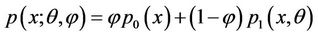
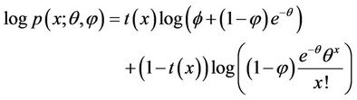
Note that the probability mass function (1.1) can be written as
 (3.3)
(3.3)
where 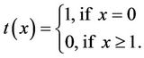
Taking log on both sides of (3.3), we get
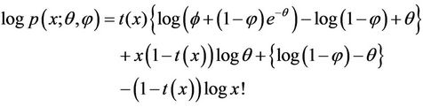
After simple rearrangement of terms, the above expression can be written as
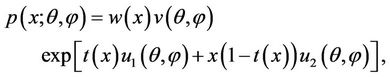 (3.4)
(3.4)
which is the general form of two parameter exponential family. Hence the zero-inflated Poisson model belongs to two parameter exponential family and thus
 (3.5)
(3.5)
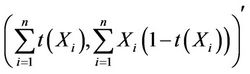
is minimal sufficient and complete for .
.
Since the ZIP model belongs to two parameter exponential family and the MMEs are based on these minimal sufficient statistics for the parameters,
where  is the Fisher information matrix and it is obtained in the next section.
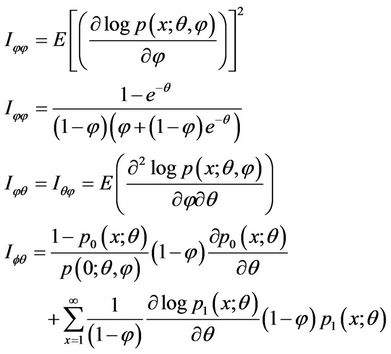
4. Fisher Information Matrix
Note that 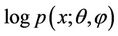 is twice differentiable w.r.t. both θ and
 .
.
Taking logarithm on both sides of (1.1), we get
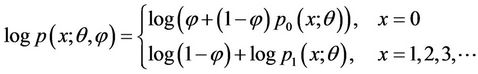 (4.1)
(4.1)
We get the following partial derivatives:
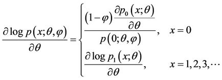 (4.2)
(4.2)
and
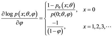 (4.3)
(4.3)
Using (4.1), (4.2), (4.3), we can verify that
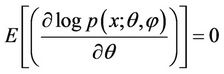
and
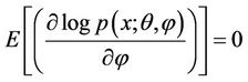
Further, we get
 (4.4)
(4.4)
On simplification, we get,
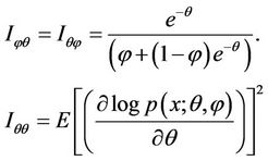 (4.5)
(4.5)
After simplification we arrive at the following expression

then
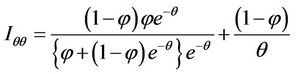 (4.6)
(4.6)
Therefore the Fisher information matrix becomes
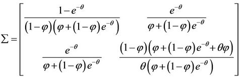 .
.
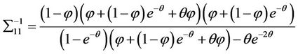
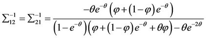
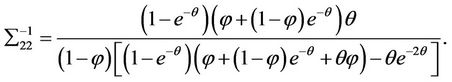
The inverse of the Fisher information matrix is
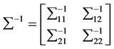
where
5. Asymptotic Relative Efficiency
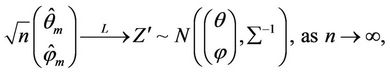
Since the MLEs of the parameters θ and  in the ZIP model have no closed form expressions, their exact standard errors are unlikely. Hence we are left with the asymptotic relative efficiencies of the estimators for the analytical comparison. Since the ZIP model in (1.1) belongs to two parameter exponential family, the MLEs of θ and
  are also asymptotically normal and
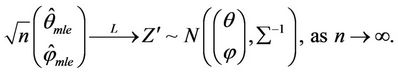
Hence the asymptotic relative efficiency of  with respect to
  is
is
Therefore, the MMEs and the MLEs of θ are asymptotically equally efficient. The same is true in the case of  too.
too.
6. Simulation Study
Using R software, 1000 samples of various sizes were simulated fixing θ = 2.5 and  = 0.3. For each of the samples the MLEs and the MMEs of θ and
  were computed. The histograms of the MLEs and the MMEs were separately drawn for θ and
 . The histograms are given in the Figures 1-4.
Nanjundan et al. [8] have carried out an elaborate simulation study by considering various values of θ and  and varying the number of samples. From the above histograms, it can be observed that the MMEs are also normally distributed even for moderate sample sizes. This gives the graphical evidence for the asymptotic normality of the MLEs and the MMEs of both the parameters in the model.
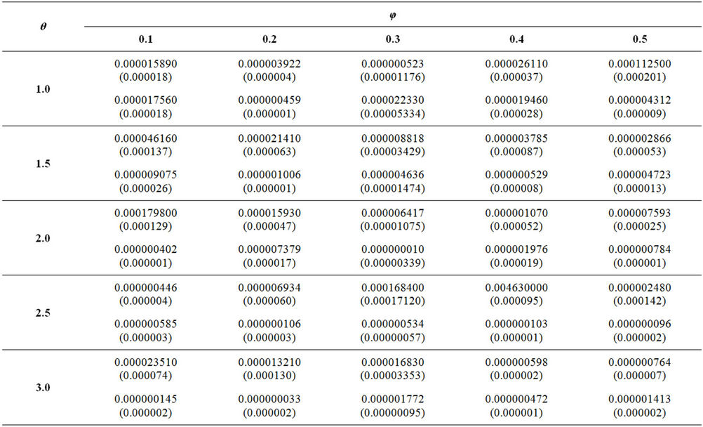
The mean squared errors (MSEs) computed from the simulation study are shown in the Appendix. The following observations about the performance of the estimates are made from the mean squared errors.
1) Though the MSEs corresponding to the MLEs are less than the MSEs of MMEs, the difference is very insignificant. That is the MMEs also perform equally good when compared the MLEs.
2) For the majority of the combinations of θ and ,
,
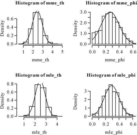
Figure 1. Histograms of the MMEs and the MLEs of θ and φ based on 1000 samples of size 25 each drawn from the distribution 0.3p0(x) + 0.7p1(x, 2.5).
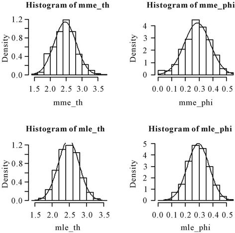
Figure 2. Histograms of the moment estimators and the MLEs of θ and φ based on 1000 samples of size 50 each drawn from the distribution 0.3p0(x) + 0.7p1(x, 2.5).
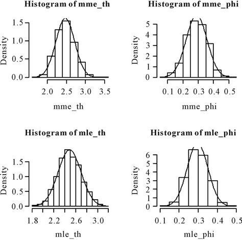
Figure 3. Histograms of the moment estimators and the MLEs of θ and φ based on 1000 samples of size 100 each drawn from the distribution 0.3p0(x) + 0.7p1(x, 2.5).
the MSEs corresponding to θ are less than the MSEs corresponding to  in the case of both the estimates.
7. Discussion and Conclusions
Zero-inflated Poisson models are readily applicable in many biological and social contexts. Two such situations are briefly discussed in this section.
Insects live on the leaves of a tree when they are found
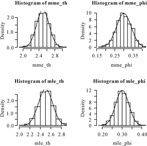
Figure 4. Histograms of the moment estimators and the MLEs of θ and φ based on 1000 samples of size 250 each drawn from the distribution 0.3p0(x) + 0.7p1(x, 2.5).
to be suitable for feeding and they do not live on those which are unsuitable for feeding. Suppose that the proportion of unsuitable leaves in a tree is  and the number of insects on a suitable leaf has a Poisson distribution with mean θ. If an observed leaf has any insects on it, then it is definitely a suitable one. On the other hand, if a leaf has no insects, then it may or may not be suitable for feeding. Let X denote the number of insects on any leaf. Then X has the p.m.f. given in (1.1).
A social group under study may have fertile and sterile couples. If the proportion of sterile couples is  and the number of children per fertile couple has a Poisson distribution with mean θ. Then X, the number of children of a randomly chosen couple, has the ZIP distribution specified in (1.1).
For more applications, one can refer to Lambert [1] and Kale [4].
The MLEs of the parameters in the ZIP model have no closed form expressions and computing them even by the EM algorithm needs computer facility. Whereas the MMEs have simple closed form expressions and they can be computed even with pocket calculators. The MMEs and the MLEs are asymptotically equally efficient. Hence MMEs can easily be used instead of the MLEs when the sample size is sufficiently large.
8. Acknowledgements
Part of this work was done during a short visit of the first author to the Dept. of Statistics, University of Poona, Pune during Jan, 2008. He is grateful to Prof. B. K. Kale for his guidance in this direction. He is also thankful to Prof. Naik Nimbalkar for providing research facility. The authors appreciate Prof. K. Suresh Chandra for useful suggestions in the presentation of the results. The authors record their deep sense of gratitude to the referee for valuable suggestions which improved the content of the paper.
REFERENCES
- D. Lambert, “Zero-Inflated Poisson Regression with an Application to Detects in Manufacturing,” Technometrics, Vol. 34, No. 1, 1992, pp. 1-14. doi:10.2307/1269547
- D.-L. Couturier and M.-P. Victoria-Feser, “Zero-Inflated Truncated Generalized Pareto Distribution for the Analysis of Radio Audience Data,” The Annals of Applied Statistics, Vol. 4, No. 4, 2010, pp. 1824-1846. doi:10.1214/10-AOAS358
- P. Yip, “Inference about the Mean of Poisson Distribution in the Presence of a Nuisance Parameter,” Australian Journal of Statistics, Vol. 30, No. 3, 1998, pp. 299-306. doi:10.1111/j.1467-842X.1988.tb00624.x
- B. K. Kale, “Optimal Estimating Equations for Discrete Data with Higher Frequencies at a Point,” Journal of the Indian Statistical Association, Vol. 36, 1998, pp. 125- 136.
- A. P. Dempster, N. M. Laird and D. B. Rubin, “Maximum Likelihood Estimation from Incomplete Data via the EM Algorithm (with Discussion),” Journal of the Royal Statistical Society: Series B, Vol. 39, No. 1, 1977, pp. 1- 38.
- G. Nanjundan, “An EM Algorithmic Approach to Maximum Likelihood Estimation in a Mixture Model,” Vignana Bharathi, Vol. 18, 2006, pp. 7-13.
- G. Nanjundan, “On the Computation of the Maximum Likelihood Estimates of the Parameters in a Mixture Model,” Mapana Journal of Sciences, Vol. 6, No. 2, 2007, pp. 57-66.
- G. Nanjundan, A. Loganathan and T. R. Naika, “An Empirical Comparison of Maximum Likelihood and Moment Estimators of Parameters in a Zero-Inflated Poisson Model,” Mapana Journal of Sciences, Vol. 8, No. 2, 2009, pp. 59-72.
Appendix
In the following table, the upper and the lower cells give the mean squared errors of the MLEs of θ and φ respectively. The values within the brackets are the mean squared errors corresponding to MMEs. Sample size = 100 and number of samples = 1000.