Applied Mathematics
Vol.5 No.15(2014), Article
ID:48888,12
pages
DOI:10.4236/am.2014.515230
Evolution of Generalized Space Curve as a Function of Its Local Geometry
Nassar H. Abdel-All1, Samah G. Mohamed1, Mariam T. Al-Dossary2
1Mathematics Department, Faculty of Science, Assiut University, Assiut, Egypt
2Mathematics Department, Girls College of Science, University of Dammam, Dammam, KSA
Email: samah_gaber2000@yahoo.com
Copyright © 2014 by authors and Scientific Research Publishing Inc.
This work is licensed under the Creative Commons Attribution International License (CC BY).
http://creativecommons.org/licenses/by/4.0/


Received 19 May 2014; revised 28 June 2014; accepted 11 July 2014
ABSTRACT
Kinematics of moving generalized curves in a  -dimensional Euclidean space is formulated in terms of intrinsic geometries. The evolution equations of the orthonormal frame and higher curvatures are obtained. The integrability conditions for the evolutions are given. Finally, applications in
  are given and plotted.
Keywords:Inelastic Curve, Curve Flow, Evolution of Curves

1. Introduction
The flow of a curve is called inelastic if the arclength of this curve is preserved. Inelastic curve flows have an importance in many applications such as engineering, computer vision [1] [2] , computer animation [3] and even structural mechanics [4] . Physically, inelastic curve flows give rise to motion which no strain energy is induced. There exist such motions in many physical applications. G. S. Chirikjian and J. W. Burdick [5] studied applications of inelastic curve flows. M. Gage, R. S. Hamilton [6] and M. A. Grayson [7] investigated shrinking of closed plane curves to a circle via the heat equation. Also, D. Y. Kwon and F. C. Park [8] [9] derived the evolution equation for an inelastic plane and space curve. Latifi et al. [10] studied inextensible flows of curves in Minkowski 3-space.
The connection between integrable systems and differential geometry of curves and surfaces has been important topic of intense research [11] [12] . Goldstein and Petrich [13] showed that the celebrated mKdV equation naturally arises from inextensible motion of curves in Euclidean geometry. Nakayama, Segur and Wadati [14] set up a correspondence between the mKdV hierarchy and inextensible motions of plane curves in Euclidean geometry. Integrable systems satisfied by the curvatures of curves under inextensible motions in projective geometries are identified in [15] . Inextensible flows of curves in Galilean space are investigated in [16] .
In this paper, we shall present a general formulation of evolving generalized curves in . The outline of this paper is as follows: In Section 2, we give the local differential geometry of curves in
 . In Sections 3 and 4, we describe the motion of generalized curves in
 . In Section 5, the integrability conditions for the considered model are obtained.
In Section 6, we specialized the motion of curves
. In Section 5, the integrability conditions for the considered model are obtained.
In Section 6, we specialized the motion of curves  to motion of plane curves (curves in
 ). Finally, Section 7 is devoted to conclusion.
2. Geometric Preliminaries
A generalized curve in a  -dimensional Euclidean space
  can be regarded as a Riemannian submanifold of dimension 1 in
  [17] .
Definition 1 A differentiable manifold of dimension 1 immersed in  is a topological hausdorff space
  with a differentiable structure
  with dimension one, where
  is an open interval in
  and
and  is a diffeomorphism mapping:

and  belongs to some index set
 .
.
Definition 2 A Generalized curve  in
in  is an image of a diffomorphism
 , where
  is an open interval of
 . The representation of
  in
in  is given by
 (1.1)
(1.1)
where  is called the parameter of the curve
 .
.
The representation (1.1) is called the regular parametric representation of  in
in , when

Also  represents an immersion in
  if
if , the parameter
 , in this case, is called the arclength parameter and is denoted by
 ,
,  is called arclength parametrization.
Frenet Frame
A Frenet frame is a moving reference frame of  orthonormal vectors
  which are used to describe the curve locally at each point
 . It is the main tool in differential geometric treatment of curves as it is far easier and more natural to describe the local properties (e.g. curvature and torsion) in terms of local reference system than using a global one like the Euclidean coordinates.
Give a curve  in
in  which is regular of order
 . The Frenet frame for the curve is the set of orthonormal vectors (Frenet vectors)
 , and they are constructed from the derivatives of
 , which are linearly independent vectors,
 .
.
Using the Gram-Schmidt orthogonalization algorithm which convert linearly independent vectors
 into the orthonormal one
  as follows:

where

By this way, one obtain an orthonormal  -tuple of vectors at
 , called the Frenet
  -frame associated with the generalized curve at the point
 , with
  is of class
  if
if . The derivatives of the frenet
  -frame at
  satisfy the following Frenet formulas:
 (1.2)
(1.2)
where  These equations can be written in a matrix form:
 (1.3)
(1.3)
where
 (1.4)
(1.4)
and  are higher curvature functions or Euclidean curvatures of the curve. The
  -th Euclidean curvature
  gives the speed of rotation of the osculation
  -plane around the osculating
  -plane.
3. Dynamics of Curves in 
Consider a smooth curve in  -dimension space. Assume that
  is the parameter along the curve in
 . Let
. Let  denotes the position vector of a point on the curve at time
 . The metric on the curve is:
 (1.5)
(1.5)
The arclength along the curve is given by:
 (1.6)
(1.6)
we use  as coordinates of a point on the curve. At
 , consider the orthonormal frame
  such that
  is the tangent vector and
  denote the normal vectors at any point on the curve.
Dynamics of the curve in  (motion of a point on the curve) can be specified by the form:
 (1.7)
(1.7)
where  are the velocities along the frame
 . Consider a local motion that is the velocities
  depend only on the local values of the curvatures
 .
.
Lemma 1 The evolution equation for the metric  is given by:
 (1.8)
(1.8)
Proof 1 Take the  derivative of (1.5) and
  derivative of (1.7), and since
 ,
,  commute, then we have:

Using (1.2), then we have

where,
 (1.9)
(1.9)
Then

Hence the lemma holds.
Lemma 2 For a simple closed curve, the evolution of the length of the curve is given by:

Proof 2 From the definition of the length , we have
 (1.10)
Substitute from (1.8) into (1.10), then the lemma holds.
4. Main Results
Definition 3 An inelastic curve is a curve whose length is preserved, i.e., it doesn't evolve in time.
 (1.11)
The necessary and sufficient conditions for inelastic flow are then given by the following theorem:
Theorem 1 The flow of the curve is inelastic if and only if 
Proof 3  Assume that the curve is inelastic.
From (1.6), the variation of the arclength is
 (1.12)
Substitute from (1.8) into (1.12), then

Since the curve is inelastic, so , hence

 Assume that
  Substitute from this equation into (1.8), so
 , then
 , this means that the arclength of the curve is preserved, hence the curve is inelastic.
Theorem 2 Consider an elastic curve . For the curve flow
 , then 1) The evolution for the frame
 , can be given in a matrix form:
 (1.13)
where  is the evolution matrix and it takes the form:

where the elements of the matrix  are given explicitly by:
 (1.14)
2) The evolution equations for the curvatures take the form:
 (1.15)
Proof 4 Consider the elastic curve  i.e.,
i.e., . Take the
  derivative of (1.7), then we have:
 (1.16)
Since , take the
  derivative of this equation, then we have
 (1.17)
Since
 (1.18)
Substitute from (1.9), (1.16) and (1.17) into (1.18), then we have
 (1.19)
Take the  derivative of (1.19), then we have:
 (1.20)
Since , take the
  derivative of this equation, then we have
 (1.21)
Since
 (1.22)
Substitute from (1.20) and (1.21) into (1.22), then we have
 (1.23)
Since , take the
  derivative of this equation, then we have
 (1.24)
Take the  derivative of (1.23), then we have
 (1.25)
Since
 (1.26)
Substitute from (1.24) and (1.25) into (1.26), and use the first equation of (1.23), then we have
 (1.27)
Take the  derivative of the second equation of (1.27), then we have
 (1.28)
Since , take the
  derivative of this equation and use the first equation of (1.27), then we have
 (1.29)
Since
 (1.30)
Substitute from (1.28) and (1.29) into (1.30), then we have
 (1.31)
By using the mathematical induction, we can extend the previous results to  -dimensional space as follows:

where , and
, and
 (1.32)
We can rewrite (1.9) and the third equation of (1.23), (1.27) and (1.31) as follows:
 (1.33)
Hence
 (1.34)
So we can rewrite (1.32) in the following form:
 (1.35)
By using the mathematical induction, we can extend the results in the first equation of (1.23), (1.27) and (1.31) as follows:
 (1.36)
Hence the theorem holds.
Lemma 3 If the curve flow (1.7) is inelastic, then the evolution equations for curvatures (1.36) take the form:
 (1.37)
Proof 5 If the curve flow (1.7) is inelastic, then
 (1.38)
Then, substitute from (1.38) into (1.36), then the lemma holds.
5. Integrability Conditions
Theorem 3 The curve  is inelastic curve
  if and only if the integrability condition (sometimes called the zero curvature condition) is given by:
 (1.39)
where  is the Lie bracket.
Proof 6 Consider the Frenet frame  that satisfy (1.4) and (1.35). Since
 (1.40)
Take the  derivative of (1.40) and use (1.13), then we have
 (1.41)
Differentiating (1.13) with respect to  and use (1.40), then
 (1.42)
From (1.41) and (1.42), then
 (1.43)
 First, If the curve is inelastic, so
  and
and  and
and  commute, then
 , hence

 Second, Assume that the integrability condition (the zero curvature condition) is satisfied, then
 (1.44)
From (1.4) and (1.35), we have
 (1.45)
Differentiating (1.4) with respect to  and (1.35) with respect to
  and use (1.36), then we have
 (1.46)
Substitute from (1.45) and (1.46) into (1.44), then we have
 (1.47)
Hence

Since  for
for . Then
 . Hence
 ,
,  i.e., the arclength is preserved. Hence the curve is inelastic.
Theorem 4 In  -dimensional Euclidean space, consider inelastic curve
 . If the matrices
  and
and  are abelian, then the elements in the evolution matrix
  take the form:

Proof 7 Since the matrices  and
and  are abelian, so
 , then the integrability condition (1.39) takes the form:
 (1.48)
Since the curve is inelastic, so , then
 (1.49)
Substitute from (1.49) into (1.48), then for![]() , we have
, we have

By using the mathematical induction, we can extend the previous results to  -dimensional space, then we have

6. Applications
Here we give some applications for time evolution equations for plane curve. We are in a position to derive time evolution of geometrical quantities. For![]() , and from (1.13), we have motion of the Frenet frame of the curve in the plane.
, and from (1.13), we have motion of the Frenet frame of the curve in the plane.
Lemma 4 In  -dimensional Euclidean space, consider an elastic curve
 . The time evolution equation for the frame
  is given by

where,

Lemma 5 The time evolution equation for the curvature of the curve in  is given explicitly by
 (1.50)
This equation represents a quasilinear parabolic partial differential equation (PDE). This result coincide with [18] .
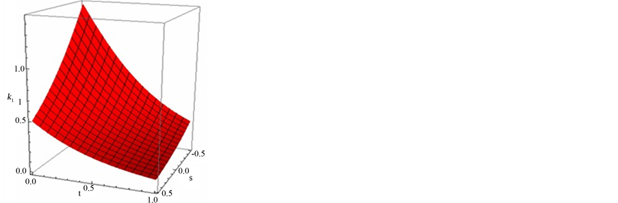
Example 1 If

Then (1.50) takes the form:
 (1.51)
The solution of the PDE (1.51) is

where  is constant. The curvature
  of the curve is plotted as a function of
  and
and  (Figure 1(a)), and for different values of
 , the curvature
  is plotted (Figure 1(b)).
Example 2 If

Then (1.50) takes the form:
 (1.52)
The solution of the PDE (1.52) is

where  and
and  are constants. The curvature
  of the curve is plotted as a function of
  and
and  (Figure 2(a)), and for different values of
 , the curvature
  is plotted (Figure 2(b)).
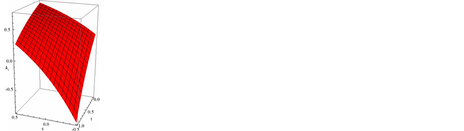
Example 3 If

Then (1.50) takes the form:
 (1.53)
The solution of the PDE (1.53) is

where  and
and  are constants. The curvature
  of the curve is plotted as a function of
  and
and  (Figure 3(a)), and for different values of
 , the curvature
  is plotted (Figure 3(b)).
 (a)
(a)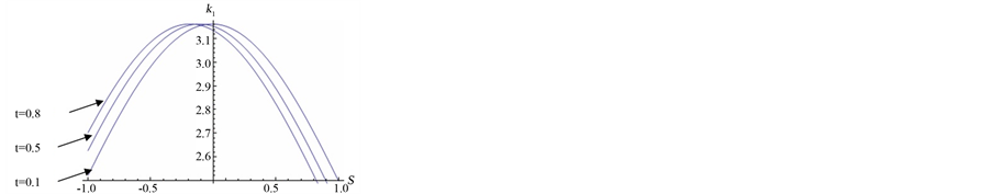 (b)
(b)
Figure 1. The curvature of the curve for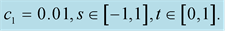
 (a)
(a) (b)
(b)
Figure 2. The curvature of the curve for
 (a)
(a)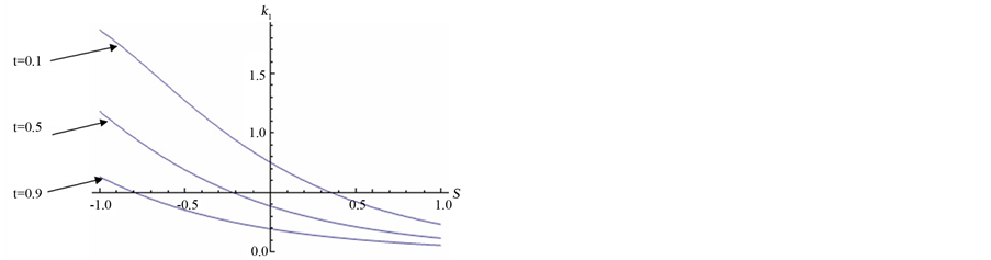 (b)
(b)
Figure 3. The curvature of the curve for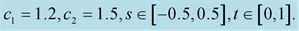
7. Conclusion
In this paper, we have discussed the motion of curves in  -dimension Euclidean space. We derived the evolution equations of the orthonormal frame and evolution equations for the higher curvatures. We get the integrability conditions for the evolutions. Moreover, we give some examples of motions of elastic curves in the plane.
Acknowledgements
The authors would like to thank the referee for helpful suggestions which improve the presentation of this work.
References
- Lu, H.Q., Todhunter, J.S. and Sze, T.W. (1993) Congruence Conditions for Nonplanar Developable Surfaces and Their Application to Surface Recognition. CVGIP, Image Understanding, 58, 265-285.http://dx.doi.org/10.1006/ciun.1993.1042
- Kass, M., Witkin, A. and Terzopoulos, D. (1987) Snakes: Active Contour Models. Proceedings of the 1st International Conference on Computer Vision (ICCV’87), London, June 1987, 259-268.
- Desbrun, M. and Cani, M.P. (1998) Active Implicit Surface for Animation. Proceedings of the Graphics Interface 1998 Conference, Vancouver, 18-20 June 1998.
- Unger, D.J. (1991) Developable Surfaces in Elastoplastic Fracture Mechanics. International Journal of Fracture, 50, 33-38. http://dx.doi.org/10.1007/BF00032160
- Chirikjian, G.S. and Burdick, J.W. (1990) Kinematics of Hyper-Redundant Manipulators. Proceeding of the ASME Mechanisms Conference, Vol. 25, Chicago, 16-19 September 1990, 391-396.
- Gage, M. and Hamilton, R.S. (1986) The Heat Equation Shrinking Convex Plane Curves. Journal of Differential Geometry, 23, 69-96.
- Grayson, M.A. (1987) The Heat Equation Shrinks Embedded Plane Curves to Round Points. Journal of Differential Geometry, 26, 223-370.
- Kwon, D.Y. and Park, F.C. (1999) Evolution of Inelastic Plane Curves. Applied Mathematics Letters, 12, 115-119.http://dx.doi.org/10.1016/S0893-9659(99)00088-9
- Kwon, D.Y., Park, F.C. and Chi, D.P. (2005) Inextensible Flows of Curves and Developable Surfaces. Applied Mathematics Letters, 18, 1156-1162. http://dx.doi.org/10.1016/j.aml.2005.02.004
- Latifi, D. and Razavi, A. (2008) Inextensible Flows of Curves in Minkowskian Space. Advanced Studies in Theoretical Physics, 2, 761-768.
- Bobenko, A., Sullivan, J., Schröder, P. and Ziegler, G. (2008) Discrete Differential Geometry. Oberwolfach Seminars, Vol. 38, X+341 p.
- Rogers, C. and Schief, W.K. (2002) Bäcklund and Darboux Transformations. Geometry and Modern Applications in Soliton Theory. Cambridge Texts in Applied Mathematics, Cambridge University Press, Cambridge.
- Goldstein, R.E. and Petrich, D.M. (1991) The Korteweg-de Vries Hierarchy as Dynamics of Closed Curves in the Plane. Physical Review Letters, 67, 3203-3206. http://dx.doi.org/10.1103/PhysRevLett.67.3203
- Nakayama, K., Segur, H. and Wadati, M. (1992) Integrability and the Motion of Curves. Physical Review Letters, 69, 2603-2606. http://dx.doi.org/10.1103/PhysRevLett.69.2603
- Li, Y.Y., Qu, C.Z. and Shu, S. (2010) Integrable Motions of Curves in Projective Geometries. Journal of Geometry and Physics, 60, 972-985. http://dx.doi.org/10.1016/j.geomphys.2010.03.001
- Ögrenmis, A.O. and Yeneroglu, M. (2010) Inextensible Curves in the Galilean Space. IJPS, 5, 1424-1427.
- Do Carmo, M.P. (1976) Differential Geometry of Curves and Surfaces. Englewood Cliffs, New Jersey.
- Nakayama, K. and Wadati, M. (1993) Motion of Curves in the Plane. Journal of the Physical Society of Japan, 62, 473-479. http://dx.doi.org/10.1143/JPSJ.62.473