Open Journal of Applied Sciences
Vol.3 No.1(2013), Article ID:29566,10 pages DOI:10.4236/ojapps.2013.31020
Electrical Resistivity Imaging of Suspected Seepage Channels in an Earthen Dam in Zaria, North-Western Nigeria
1Department of Mathematics, Statistics and Computer Science, College of Science and Technology, Kaduna Polytechnic, Kaduna, Nigeria
2Department of Physics, Kogi State University, Anyigba, Nigeria
Email: bedrock969@yahoo.com
Received November 6, 2012; revised December 7, 2012; accepted December 14, 2012
Keywords: Anomalous Seepage; Earthen Dam; Unconsolidated Formations; Loose Ground; Saturated Zones
ABSTRACT
To determine and map the subsurface conditions of a dam, a 2D electrical resistivity tomography study was carried out within the two flanks of Zaria dam at Shika. This was done to ascertain if the variations in the volume of water content in the dam is due to an anomalous seepage beneath the subsurface or seasonal effects. On the basis of the interpretation of the acquired data, various zones of relatively uniform resistivity values were mapped and identified. The first zone is characterized by moderate resistivity values of 150 - 600 ohm-m. It represents unsaturated topsoil with thicknesses varying from 1 - 4.5 m. The second (intermediate depth) resistivity zone, with values ranging from 5 - 100 ohm-m and thickness varying from 3.5 - 10 m, represents a silt clay layer with high moisture content. The third resistivity zone represents fairly weathered granite and is characterized by relatively high resistivity values ranging from 700 - 6000 ohm-m. The available borehole log data correlated well with the pseudo-sections in relation to the obtained resistivity values and depth. Zones of relatively low resistivity within the bedrock are interpreted to represent potential seepage pathways. Hence, this geophysical method can be successfully used to delineate and map these seepage pathways within the subsurface of the earth dam.
1. Introduction
Electrical resistivity is one of the most sensitive geophysical methods for monitoring changes of electrical properties in the subsurface. Some applications of 2D inversions have provided reliable models for the subsurface such as Loke and Baker [1,2] amongst others. It is very effective in determining depth to water saturated zone and groundwater flow pattern [3,4]. The resistivity of soils is dependent on saturation, porosity, permeability, ionic content of the pore fluids, and clay content. In the case of water seepage through a dam, it can be detected as resistivity low using electrical resistivity methods [5,6]. In spite of the distortion of apparent resistivity data caused by the topography and variation of electrical properties, using the resistivity method along the flanks of a dam is a practical and favorable tool to detect leakage zones. The data acquisition is nondestructive and convenient. In either case, a seepage assessment program may be necessary to detect and map seepage paths and determine if remedial measures are necessary to abate the seepage. Previous geophysical studies have demonstrated the utility of using electrical resistivity methods to detect and characterize the seepage conditions occurring at dams [7]. Dahlin and Johansson [8], Johansson and Dahlin, [5], Aal et al. [6] and Cho and Yeom [9], had earlier applied this method to study the embankment of dams. Benson et al. [10] had also applied it successfully to the detection of buried wastes and wastes migrations. On the other hand, Osazuwa and Chinedu [11] had earlier investigated and mapped the high permeability zones beneath the same dam using Seismic Refraction Tomography. Their results showed the existence of depressions and low velocity zones indicating the presence of loose and unconsolidated materials beneath the flanks of the dam. This study intends to confirm this results using electrical resistivity method. Although this study was carried out at a different time using a different profiling geometry, the objective was to detect the potential seepage paths and assess conditions of the foundation at the dam with Electrical Resistivity Tomography (ERT) method. It will also aid to determine whether the seepage is associated with the nature of earth materials used for the dam construction or resulting from the existence of loose and unconsolidated formations beneath the dam. Therefore, detection and characterization of loose and unconsolidated formations which may be a source of water loss from the dam through seepage, is highly necessary, in order to prevent structural failure of the dam. Most importantly, it is intended to provide complementary information about the subsurface as discussed in Osazuwa and Chinedu [11].
2. Location and Geology of the Study Area
This study was carried out at approximately latitude 11˚00'N and 11˚08'N and longitude 7˚45'E and 8˚00'34''E (Figure 1). The area [12,13] is dominantly of older laterite which are mainly red, homogeneous porous rocks reduced to the present red mesas form which is approximately 6 - 20 m above present ground level. A younger laterite, up to 2 meters, is often found along present river valleys, both underlain and overlain by alluvium and local discontinuities marked by sand rivers [12]. Thin discontinuous sand deposits are found in the smaller streams and upper reaches of larger river valleys, while more extensive deposits of grey-brown sands, silts and clay are present along most of these rivers [14].
3. Data Acquisition
Electrical resistivity methods involve the measurements of the apparent resistivity of soils and rocks as function of depth or position. The traditional four-electrode resistivity configurations as described in, Dobrin and Savit, [15] and Telford et al. [16], have been confirmed inadequate [1,3,4,17]. Therefore in this study, the field procedure as described in Loke [3,4] was adopted.
Measurements were made using (42) forty two electrodes connected by multi-core cable to the ABEM Terrameter SAS 4000/1000 with LUND Imaging System. We adopted the sequence of measurements as described in Loke [3,4], Loke and Baker [1,2], with electrodes stuck in a straight line with constant spacing (Figure 1).
The electrodes coverage along a straight line spans 200 m and no change of resistivity in the direction that is perpendicular to the survey line was assumed [3]. In order to overcome the problem of limited number of electrodes and ensure a better coverage, a roll along technique was adopted [3,4], except along the profile where physical limitations or obstacles encountered in the survey area could not permit. Profiles were taken along the field profile geometry as shown in Figure 1. The profiles were planned parallel to the dam flanks in order to delineate possible micro-structures or features within the area. It was possible to carry out a roll-along method in profiles P1, P2 and P3, while P4 was inhibited to just single spread by relics of fallen building in the area. Each profile array showed advantage and disadvantage in terms of depth of investigation, sensitivity to horizontal or vertical variations and signal strength. Following the extent of dryness of the ground as at the time of this survey, electrodes were placed in shallow holes wetted with salty water to ensure proper contact impedance with the ground and reduce the source of noise from the lake and topsoil [6]. A constant spacing of 5 m between adjacent electrodes was used, while the multi-core cable was attached to an electronic switching unit. The Wenner method was adopted, whose format for the control file is described in Loke [4] and the manual according to GEOTOMO SOFTWARE [18]. The multi channel adapter (electrode selector) was used to connect more than one potential and current electrode channels in Vertical Electrical Sounding.
4. Data Processing
The acquired data were processed with RES2DINV program developed by Loke and Barker [1], Geotomo Software [18] and modified by Loke [4], which will automatically determine a two dimensional resistivity model for the subsurface. Normally, the data from the surveys conducted at different times were inverted independently, frequently with a smoothness-constrained least-squares inversion method [19]. The inverted resistivity distribution can also give important information about the location of leakage zones in the vertical section. The resistivity of the ground depends mainly on the porosity, water saturation, and clay content. This is based on the fact that an increase in the porosity typically leads to increase in water content, which reduces the electrical resistivity [4,18]. A porosity increase also leads to greater permeability, and this affects the increased seepage flow. The aim of this study is to confirm that the electrical resistivity method is effective in detecting the zones prone to leakage. A 2D electrical resistivity survey using the Wenner array is useful for delineating the leakage pathways since leaks generate strong high conductive anomalies.
5. Inversion
Solving an inverse problem means to infer the values of the model parameters from given observed values of the observable parameters [20]. In order to understand the earth’s interior, geophysicists had to develop the inverse problem theory in order to use the set of data collected at the surface to model that of the interior. Loke [4] explained that in geophysical inversion, we seek to find a model that gives a response similar to the actual measured values. The model is an idealized mathematical representation of a section of the earth. It has a set of model parameters that are the physical quantities we
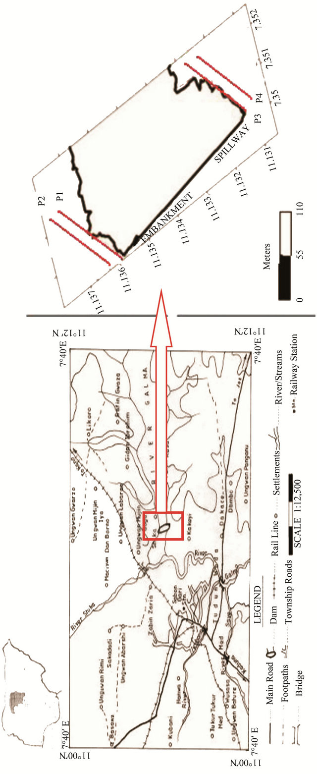
Figure 1. The topography map (McCurry, 1973) showing the survey area. Insert, on the right, is the GPS mapped profile geometries of the geophysical surveys on both flanks of the dam.
want to estimate from the observed data. The model response is a synthetic scenario that can be calculated from the mathematical relationships defining the model for a given set of model parameters. All inversion methods essentially try to determine a model for the subsurface whose response agrees with the measured data subject to certain constraints. The empirical method of inverting measured apparent resistivity data includes plotting the resistivity data on a log-log graph paper. The interpretation usually assumes that the subsurface resistivity changes only with depth (in vertical direction), but does not change laterally. This method of inverting measured apparent resistivity data usually reproduces a one dimensional model which drives the interpretation of the subsurface. Inherent problems obtainable in one-dimensional methods of processing and interpretation of geophysical data include the misinterpretation of changes in apparent resistivity, caused by lateral changes in subsurface resistivity and non uniqueness of the resultant model. Moreover, topography can also influence electrical surveys as current flow lines to follow the ground surface, thus equipotential surface are distorted and anomalous readings can result. It is nowadays possible to invert the data into a full two-dimensional geoelectrical model [1,2], rather than a sequence of discrete, one dimensional geoelectrical sections. To determine the resistivity distribution from measurements of potential differences is a non unique problem and its numerical solution is unstable: small variations in the data can cause large variations in the solution. Commonly used inversion methods provide unique and stable solutions by introducing the appropriate stabilizing function [21]. The main aim of the stabilizer is to incorporate a priori knowledge in the inversion process. ERT is a typical example of ill-posed problem. Regularization is the most common way to solve this kind of problems. It basically consists in using a priori information about targets to reduce the ambiguity and the instability of the solution. Two dimensional Inversion of a geophysical data set results in a model of the resistivity characteristics of the subsurface; in this case, a model of the electrical properties of the subsurface. The inversion routine is based on the smoothness-constrained least squares method [4,19] and can be used for many electrode configurations, including those used in this study. Loke [3] confirmed that optimization method tries to reduce the difference between the calculated and measured apparent resistivity values by adjusting the resistivity of the model blocks subject to the used smoothness constraints. A measure of this difference is given by the root-mean-squared (RMS) error. However, according to Loke [3] the model with the lowest possible RMS error can sometimes show large and unrealistic variations in the model resistivity values and might not always be the “best” model from a geological perspective. In general the most prudent approach is to choose the model at the iteration after which the RMS error does not change significantly. It is noteworthy that the software has a facility for editing or removing any bad data point. The main purpose of this option is to remove data points that have resistivity values that are clearly wrong. Such bad data points could be due to the failure of the relays at one of the electrodes, poor electrode ground contact due to dry soil, or shorting across the cables due to very wet ground conditions. These bad data points usually have apparent resistivity values that are obviously too large or too small compared to the neighboring data points. The best way to handle such bad points is to eliminate them so that they do not influence the model obtained. Meanwhile, the true resistivity of the subsurface is then determined from the apparent resistivity measurements. One method that is widely used is the linearised smoothness-constrained least-squares optimization method where the relationship between the data and model parameters is given in Loke and Barker [1,2].
6. Results and Interpretation
The pseudosection and inversion models are useful means of presenting the measured apparent resistivity values in a pictorial form, and as an initial guide for further quantitative interpretation. Different arrays used to map the same region can give rise to very different contour shapes in the pseudosection plot. It can also give an idea of the data coverage that can be obtained with different arrays. The nearest available three borehole log data are used as control over the interpretation of the resistivity pseudosections (Table 1) as done in Osazuwa and Chinedu [11]. It is always necessary to consider further exploratory geophysical results gathered from the surface with borehole log data. This is to reduce the site characterization cost and establish the most useful locations for geological or geotechnical samples [21]. The results obtained based on 2D inversion of field data and borehole information, were interpreted to determine the depth and extent of shallow bedrock, thickness of overburden, aquifer etc. The results of the 2D electrical resistivity profiles acquired on the two flanks of Zaria dam, Shika are shown in Figures 2-5. Figure 2 shows the resistivity Pseudosections and inverse model of profile one (P1) acquired on the edge of the northwestern flank of the dam. It is one of the closest to the dam reservoir and shows a top layer resistivity value range of between 15 Ωm and 989 Ωm. The electrical imaging as shown in Figure 2 surprisingly showed that this area is further composed of partly saturated but compacted materials that gave rise to a high resistivity value of 433 Ωm and 2261 Ωm in the top layer. The electrical resistivity inverse model of this same profile showed some areas of
Table 1. The results of electrical resistivity and depths correlated with three available boreholes log data [23].
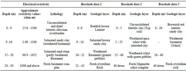
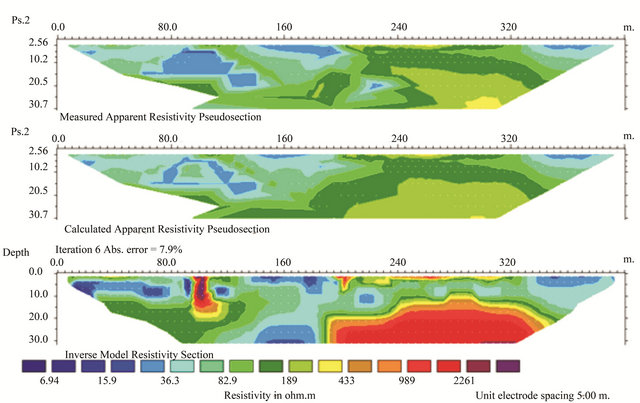
Figure 2. Measured, calculated and Inverted model apparent resistivity imaging with the Pseudosections for profile 1 (P1).
high resistivity zones in the overburden probably due to compactness and dryness around the dam. However this may have also contributed to high resistivity values in the overburden. The dryness and compactness of the topsoil may be due to evapo-transpiration and/or animal movements that may lead to consolidation. However, there are zones of low apparent resistivity values indicating the presence of potential seepage paths with the subsurface. The saturated zones on the top layer of this profile may probably be attributed to excessive water contents due to irrigation or reservoir overflow.
|
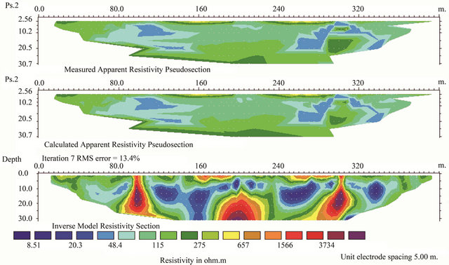
Figure 3. Measured, calculated and Inverted model apparent resistivity imaging with the Pseudosections for profile 2 (P2).
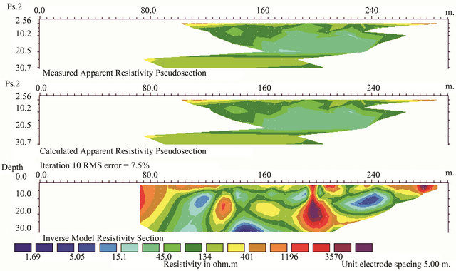
Figure 4. Measured, calculated and Inverted model apparent resistivity imaging with the Pseudosections for profile 3 (P3).
a depth ranges from 10 m to 30 m from the crest of the dam and represents the granitic bedrock. The anomalous low resistivity zones exist between 100 m and 200 m electrode positions on the profile line. The hanging structure with high resistivity values of 1566 Ωm and 3734 Ωm, as thrusting downward to the basement has discontinuities at approximately between 3 m to 10 m depth by the eastern part of the profile (P1) and extended down to 20 m at the western side of the profile. They continued as diapiric structures from the basement, looking like outcrops at exactly 95 m and 100 m on the western side of the profile, and 300 m and 310 m on the eastern side of the profile. These may probably be either part of the dam’s construction plan or any other feature that
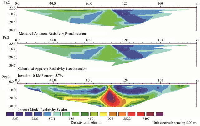
Figure 5. Measured, calculated and Inverted model apparent resistivity imaging with the Pseudosections for profile 4 (P4).
might not have a relative geologic interpretation. These features may be a zone of the dam filled with compacted, consolidated and dried laterite or any other geologic material for a special purpose, since Zaria dam at Shika is a Zoned earthen dam. It was rather not detected on the corresponding profile two (P2). None of the previous discontinuities were found on profile two (P2) (Figure 3), yet it showed some similarities to profile one (P1). There are features of anomalous low resistivity zones of 8.51 Ωm - 48.4 Ωm below 10 m depth down to the bedrock. These features can be as a result of excessive weathering or fracturing of the bedrock within the area. However it is in good agreement with profile 2 of the seismic refracttion tomography result of Osazuwa and Chinedu [11] where the same feature existed as depression below the 10 m depth of the profile.
Profile three (P3) (Figure 4) is shown to be adversely affected by the dryness of the ground, which makes movement of ions within the subsurface difficult. This affected the resistivity readings through the electrodes in the western part of the profile to about 70 m of the entire profile since measurements may be limited by either highly conductive or highly resistive surface soils.
If shallow clays and extremely shallow groundwater are present, most of the current may concentrate at the surface. Although the condition is very rare, the presence of thick, dry, gravelly material (or massive dry material) at the surface may prevent the current from entering the ground. This profile is dominantly made up of pockets of fairly saturated zones or saturated clay lenses, and highly dried zones. It can be attributed to the position of this profile, being at about 150 m from the dam reservoir. The resistivity ranges characterizing the bedrock (300 Ωm to 4500 Ωm) is also observed in this resistivity profile. A moderate resistive layer, 1.69 Ωm - 400 Ωm is observed within this isolated profile. This layer may represent highly weathered or dissolved bedrock materials. Moreover, the resistivity model and Pseudosections of profile two (P2) and three (P3) show a change in the bedrock pattern and an anomalous low resistivity zone (1 - 40 Ωm) located within moderate resistivity zone of the weathered or fractured bedrock described above (Figures 3 and 4). This anomalous low resistivity zone may represent a flow channel for groundwater. It is clear that the depth to bedrock is lower or shallow in this profile. The observed shallowness of the bedrock allows the conduit formed by the bedrock weathering or dissolution to intersect with ground surface further forming the observed seepage path. The diagonally vertical structure featuring in profile four (P4) at a horizontal distance of between 80 m to 120 m and also existed at profile three P3 between 195 - 205 m, may be a compacted laterite formation used also in the dam construction. The resulting model from the inversion (Figure 5) shows three distinct areas of very high apparent resistivity (>1000 Ωm) at approximately 50 m to 135 m horizontal distance and at about 15 m depth, the high resistive feature outcropping at approximately 100 m to 105 m, may be part of the mapped dam construction.
There are anomalous saturated areas at 1.5 m to 14 m depth and spans through the entire profile horizontally, spanning up to 65 m length (105 m - 170 m) horizontally. This is a probable evidence of permeable zones that conducts seepage and eventual accumulation at that level. This was slightly detected by the seismic refraction investigation in the same profile of Osazuwa and Chinedu [11]. Besides the feature of this diapiric structure, other very high apparent resistivity areas are probably related to natural geologic materials that may be interpreted as dried weathered materials. This led to the prominent feature of much dissolved bedrock materials in the weathered zone overlying the basement. However, the inverted section at the downstream slope does not show any low-resistivity zone. Intermediate resistivity values at the shallow depth of the section represent the fill material. Meanwhile, high values of resistivity at the lower depth are interpreted as the secondary influence of the foundation with high resistivity values. Generally, weathering of the granite bedrock produces a clayey and/or sandy soil mixed with granite pebbles and other partially weathered materials. This is probably caused partly by surface water accumulation due to irrigation and excessive flooding in this region, or eventual downward infiltration that reduces the resistivity to less than 600 Ωm. A thin layer of moderate resistivity ranging from low to high is observed along the top of the resistivity image. This correlates with the observed unconsolidated consolidated clay and laterite. The sand and gravel channel that runs through the cross-section corresponds with the resistivity values of the weathered materials. The bottom layer has a low to moderate resistivity of 8 Ωm to 174 Ωm and corresponds to the seepage pathway overlying the bedrock.
The diagonally vertical structure featuring in profile four (P4) at a horizontal distance of between 80 m to 120 m and also existed at profile three P3 between 195 - 205 m, may be a compacted laterite formation used also in the dam construction. The resulting model from the inversion (Figure 5) shows three distinct areas of very high apparent resistivity (>1000 Ωm) at approximately 50 m to 135 m horizontal distance and at about 15 m depth, the high resistive feature outcropping at approximately 100 m to 105 m, may be part of the mapped dam construction.
7. Discussion and Conclusions
The results from the electrical imaging survey were subsequently confirmed by boreholes. In the inversion model, a high resistivity anomaly uniformly detected below the 15 m down, is probably partly weathered to fresh basement in the survey area which is prominent around the Zaria area. This feature is in agreement with the findings of McCurry [12], Karofi [17] and Okoro [22]. In the inversion models, most of the riverbed materials have a resistivity of less than 120 Ωm. There are several areas where the near-surface materials have significantly higher resistivity of over 150 Ωm. The lower resistivity materials are possibly more coherent sediments, whereas the higher resistivity areas might be coarser and less coherent materials. From this study, it is observed that the depth of the leakage zone is below 4 m depth from the crest. Thus, the top of the leakage zone is just 2.5 m below the plane on which the survey lines are placed. Hence, leakages take place at the lower part of the dam. To detect a deeper leakage zone, a broader resistivity survey should be performed.
The comparison of the measured apparent resistivity pseudosection and the calculated apparent resistivity pseudosection resulted in a reasonably good agreement with the inverse model resistivity section. As a result, this demonstrates the stability of the 2D inversion algorithm that can give reliable models. Based on the electrical images obtained in the study area, three distinct layers were revealed. More so, various zones of relatively uniform resistivity values were identified and mapped. The first zone is characterized by moderate resistivity values of 150 Ωm - 600 Ωm. It represents unsaturated and mostly dried laterite as topsoil with thicknesses varying from 1 m to 4.5 m. The second (intermediate depth) resistivity zone, with values ranging from 5 Ωm to 100 Ωm and thickness varying from 3.5 m to 10 m, represents a silt clay layer with high moisture content. The third resistivity zone represents fairly weathered granite and is characterized by relatively high resistivity values ranging from 700 Ωm to 6000 Ωm. Zones of relatively low resistivity within the bedrock are interpreted to represent weak zones and potential seepage pathways. These exist within the overburden, weathered Basement and the fresh Basement. The Overburden is made up of two parts, the topmost of which is about 9 m thick and is composed of reddish brown lateritic clay. The second layer is about 7 m thick which is composed of brownish sandy clay. Combining these two parts together reveals an overburden with an average thickness of about 16 m - 21 m which agrees with the borehole logs (Table 1).
The Weathered Basement, which is underlying the overburden, consists of disintegrated schistose rock materials, sand and gravel. This layer has a relatively low resistivity due to the presence of water and clay, which reduces the permeability, so this layer is thus regarded as the aquifer as it usually holds water. Also, the layer is highly weathered and the degree of weathering increases toward the southern part of the study area. This increased thickness of bedrock weathering is a proof of the capability of this layer to provide a good reservoir with a higher probability of the presence of fractures in the basement. The average thickness of this layer is about 5 m - 14 m. Thus, this correlates well with the borehole logs of the site being investigated. The fresh Bedrock was encountered at a variable depth of between 20 m and >30 m respectively. The average depth of the fresh basement is about 40 m as provided by the borehole log. The value of the resistivity of the basement rocks is appreciably high, rising from 1223 Ωm up to 11918 Ωm which is indicative of typical crystalline bedrock. This layer is believed to grade indefinitely or infinitely downward. The average depth of penetration is about 29.3 m. The basement though fresh, is frequently fractured which gives it a high permeability. But as fractures do not constitute a significant volume of the rock, fractured basement has low porosity.
This study demonstrates that anomalous low resistivity zones can be attributed to areas of unconsolidated and loose ground within the overburden, which constitutes most of the high permeable channels of seepage in the area. The results from this study are in good agreement with the existing borehole data within the area. Moreoveranomalous zones of low resistivity values were observed within the aforementioned highly weathered zone and extend from the resistivity profiles existing within the 50 m from the reservoir, on the flanks of the dam, suggesting a possible conduit for water flow. Hence, the layering of the depositions in the overburden seems to be erratic, discontinuous and heterogeneous. This is in agreement with the findings of Osazuwa and Chinedu [11] using Seismic refraction tomography. The study rightly confirms that the alluvium consists of laterite, sand and gravel overlain by sandy clay, which is about 10 to 15 m thick and fills the bottom of the stream valley. Zones of relatively low resistivity within the bedrock are interpreted to represent weak formations and potential seepage pathways.
REFERENCES
- M. H. Loke and R. D. Barker, “Least-Squares Deconvolution of Apparent Resistivity Pseudosections,” Geophysics, Vol. 60, No. 6, 1995, pp. 1682-1690.
- M. H. Loke and R. D. Barker, “Rapid Least-Squares Inversion of Apparent Resistivity Pseudosections by QuasiNewton Method,” Geophysical Prospecting, Vol. 44, No. 1, 1996, pp. 131-152.
- M. H. Loke, “Electrical Imaging Surveys for Environment and Engineering Studies (A Practical Guide to 2D and 3D Surveys),” Earth Sciences, Vol. 6574525, No. 1999. www.terraplus.com
- M. H. Loke, “Tutorial: 2D and 3D Electrical Imaging Surveys,” 2004. www.geoelectrical.com
- S. Johansson and T. Dahlin, “Seepage Monitoring in an Earth Embankment Dam by Repeated Resistivity Measurements,” European Journal of Engineering and Geophysics, Vol. 1, 1996, pp. 229-247.
- G. Z. A. Aal, A. M. Ismail, N. L. Anderson and E. A. Atekwana, “Geophysical Investigation of Seepage from an Earth Fill Dam, Washington County, MO,” Journal of Applied Geophysics, Vol. 44, 2004, pp. 167-180.
- T. V. Panthulu, C. Krishnaiah and J. M. Shirke, “Detection 407 of Seepage Paths in Earth Dams Using Self-Potential and Electrical Resistivity Methods,” Engineering Geology, Vol. 59, No. 3-4, 2007, pp. 281-295. doi:10.1016/S0013-7952(00)00082-X
- T. Dahlin and S. Johansson, “Resistivity Variations in an Earth Embankment Dam in Sweden,” 1st Meeting Environmental and Engineering Geophysics, Torino, 25-27 September 1995, p. 4.
- I. Cho and J. Yeom, “Crossline Resistivity Tomography for the Delineation of Anomalous Seepage Path Ways in an Embankment Dam,” Geophysics, Vol. 72, No. 2, 2007, pp. 31-38. doi:10.1190/1.2435200
- R.C. Benson, R. Glaccum and M. Noel, “Geophysical Techniques for Sensing Buried Wastes and Waste Migration (NTIS PB84-198449),” US EPA Environmental Monitoring Systems Laboratory, Las Vegas, 1984, p. 236.
- I. B. Osazuwa and A. D. Chinedu, “Seismic Refraction Tomography Imaging of High Permeability Zones Beneath an Earthen Dam, in Zaria Area, Nigeria,” Journal of Applied Geophysics, Vol. 66, 2008, pp. 44-58.
- Y. A. Karofi, “Interim Report on the Geology of 1:100,000 Sheet 102 (Zaria),” Geological Survey of Nigeria, 1973.
- P. McCurry, “Geology of Degree Sheet 21 Zaria, Nigeria,” Overseas Geology Mineral Research, Vol. 45, 1973, p. 45.
- Water and Power Development Company (WAPDECO), “Kaduna State Water Board Rehabilitation Study, Part 1, Zaria Water Supply Scheme,” Final Report, 1991.
- M. B. Dobrin and F. Savit, “Introduction to Geophysical Prospecting,” McGraw-Hill Company Ltd., NewYork. 1988.
- W. M. Telford, L. P. Geldart and R. E. Sheriff, “Applied Geophysics,” Cambridge University Press, New York, 1990. doi:10.1017/CBO9781139167932
- D. H. Griffiths and R. D. Barker, “Two-Dimensional Resistivity Imaging and Modeling in Areas of Complex Geology,” Journal of Applied Geophysics, Vol. 29, No. 3-4, 1993, pp. 211-226. doi:10.1016/0926-9851(93)90005-J
- GEOTOMO SOFTWARE, “Rapid 2D Resistivity and IP Inversion Using the Least Squares Method. Wenner (α, β, γ), Dipole-Dipole, Inline Pole-Pole, Pole-Dipole, Equatorial Dipole Dipole, Schlumbeger and Non-Conventional Arrays,” On Land, Underwater and Cross-Borehole Surveys, 2001. www.geoelectrical.com www.terraplus.com
- C. De Groot-Hedlin and S. C. Constable, “Occam’s Inversion to Generate Smooth, Two Dimensional Models from Magneto Telluric Data,” Geophysics, Vol. 55, No. 12, 1990, pp. 1613-1624. doi:10.1190/1.1442813
- A. Tarantola, “The Inverse Theory,” Academic Press Inc., Cambridge, 1987.
- W. Zhou, F. Beck and A. Adams, “Effective Electrode Array in Mapping Karst Hazards In Electrical Resistivity Tomography, Annealing Optimization for Inversion of First Arrival Times,” Bulletin of the Seismological Society of America, Vol. 84, No. 5, 2002, pp. 1397-1409.
- A. C. Okoro, “Interim Report on the Geology of 1:100,000 Sheet 101 (Maska),” Geological Survey of Nigeria, 1973.
- National Water Resources Institute (NWRI), “Groundwater Research Development,” Completion Report, 2008, Borehole NR. GWR/HG-05(1/6).
NOTES
*Corresponding author.