Journal of High Energy Physics, Gravitation and Cosmology
Vol.05 No.03(2019), Article ID:94094,12 pages
10.4236/jhepgc.2019.53050
A Very Simple Model Concerning the Unified Field Theory Basing on the Kronig-Penney-Model
Carsten Wochnowski
Independent Researcher, Karlsfeld, Germany

Copyright © 2019 by author(s) and Scientific Research Publishing Inc.
This work is licensed under the Creative Commons Attribution International License (CC BY 4.0).
http://creativecommons.org/licenses/by/4.0/


Received: January 22, 2019; Accepted: July 28, 2019; Published: July 31, 2019
ABSTRACT
In this paper, a very simple novel model is presented concerning the unified field theory (“theory of everything”). In the scope of this novel theory, it is assumed that matter, space and time are quantized. It is assumed that the space is subdivided into cubic elementary cells (space quanta), and in each of its eight corners a Delta potential is positioned. That means the Delta potentials are equidistantly arranged, so that the Delta potentials are forming a lattice similar to a crystal lattice in solid state physics. The novel theory is analogue to the Kronig-Penney model well-known in solid state physics: a crystal lattice comprises Delta potentials arranged equidistantly to one another, so the lattice space can be considered as being quantized by an array of equally spaced Delta potentials or the lattice space is divided into cubic elementary cells (space quanta). But instead of electrons, material quanta are inserted into the cubic elementary cells or space quanta. So the material quanta are not freely vibrating (unbound state), but are vibrating in a bound state with discrete energy levels separated by an energy gap. This is due to the presence of the array of Delta potentials. In the frame of this novel theory the Schrödinger Equation for the Kronig-Penney-Model is not solved by differentiation, but the Schrödinger Equation is integrated yielding the formula , by whose discussion the existence of an energy gap is revealed. This energy gap is responsible if the material quantum occurs as light quantum (photon) or mass quantum.
Keywords:
String Theory, Loop Quantum Gravity Theory, Unified Field Theory

1. Introduction
In the frame of the unified field theory research (“theory of everything”), there exist two theories competing one another: the first one is called the string theory and the second one is called the loop quantum gravity theory.
According to the string theory the universe consists of freely vibrating objects called strings with the dimension in the order of Planck length [1] - [10] . At the moment mainly two kinds of strings are discussed: the first one comprises open strings featured by a segment with two endpoints and the second one comprises closed strings featured by a closed segment similar to a loop e.g. like a circle [11] . A further development of this theory is called Superstring theory [12] . A generalization of string theory is the so-called M-theory [13] [14] .
In 1974, K. Wilson has developed a gauge theory featured by regulisation of space and time [15] .
According to the loop quantum gravity theory, the space and time is quantized, while the space is structured by a very fine network of woven finite loops [16] [17] [18] [19] [20] .
D. Vaid has tried to combine both well-recognized theories the string theory and the loop quantum gravity theory into a common theory, so both theories are not competing one another but are completing one another [21] .
2. Theoretical Contemplation
In the scope of the novel theory it is assumed that matter is quantized. In the following this matter quantum is also called material quantum. Besides it is assumed that space is also quantized: the space is subdivided into cubic elementary cells confined by eight corners, and in each corner a Delta potential is located. That means the Delta-potentials are equidistantly arranged or the Delta potentials are forming a lattice similar to a crystal lattice in solid state physics. In the following these cubic space elementary cells are called space quanta. Also it is assumed that the time is also quantized (time quantum).
The novel theory is analogue to the Kronig-Penney model well-known in the solid state physics [22] [23] [24] : The equidistantly spaced positively charged atom cores are represented as Delta potentials, thus a crystal lattice is contemplated which contains Delta potentials arranged equidistantly to one another, so the lattice space can be considered as being quantized by an array of equally spaced Delta potentials or the lattice space is divided into cubic elementary cells (corresponding to space quanta of the novel theory). In solid state physics this yields the Schrödinger Equations as a system of coupled differential equations. The Schrödinger Equations for the Kronig-Penney-Model is solved by differentiation, that means as an approach a complex exponential function is applied yielding a dispersion function leading to the existence of an energy gap.
But by the novel theory instead of electrons, material quanta (e.g. in form of zero-dimensional punctual mass objects) are inserted into the cubic elementary cells or space quanta. So the material quanta are not freely vibrating (unbound state), but are vibrating in a bound state with discrete energy levels separated by an energy gap. This is due to the presence of the array of Delta potentials. It is important to mention that the material quanta are not considered as strings at this point.
In this case of the novel theory, instead of solving the Schrödinger Equation by differentiation the Schrödinger Equation is solved by integration, that means the Schrödinger Eqauation is integrated and yields the formula , by whose discussion the existence of an energy gap is revealed. This energy gap is responsible if the material quantum occurs as light quantum (well-known als photon) or mass quantum (until now not experimentally confirmed).
It is assumed that space is subdivided into cubic space quanta which are confined by Delta potentials in its corner points. This is equivalent with a space model traversed by an array of equally spaced (equidistant) Delta-potentials which is comparable to a common simple cubic crystal lattice with a lattice constant “a” described by the Kronig-Penney model in solid state physics. Between the Delta potentials material quanta occur which can be resting or moving with or without acceleration. The material quanta are not free or unbound but bound by the array or lattice of Delta potentials. The material quanta are described by the probability distribution : the material quanta are located either between two adjacent Delta potentials or at the site of the Delta potentials. For the purpose of simplicity it is supposed that exactly one material quantum is located between two Delta potentials, so in every cubic space quantum exactly one material quantum exists.
Thus the corresponding Schrödinger equation is as followed:
But instead of solving the Schrödinger equation by an complex exponential function leading to the dispersion relation, now the Schrödinger equation is integrated from −∞ to +∞ after having been multiplied with the complex conjugated :
In consideration of , the normalization , the definition of the Dirac Delta distribution and the assumption that is overall a steady and differentiable function, a short calculation yields the formula:
or
Now it is assumed that between every two adjacent Delta potentials exactly one material quantum is located. So due to (summarization above all Delta potentials):
This formula can be interpreted as follows: the probability density of a material quantum at the Delta-potential is maximum, if the kinetic energy is zero, while the material quantum probability density at the Delta-potential is minimum, if the total energy E is equal to the kinetic energy Ekin.
Now the material quantum probability density is drawn against the kinetic energy Ekin, thus due to this yields a linear graph with a negative slope and with a y-intercept as shown in Figure 1.
Thus we discuss the graph as follows: the zero point of the graph (point of intersection between the graph and x-coordinate (axis of abscissae)) is denoted as E0, then the physically reasonable solutions are located in the area between between the minimal kinetic energy Ekin = 0 (the kinetic energy Ekin is zero) and the maximal kinetic energy Ekin = E = E0 (kinetic energy Ekin is equal to the total energy E). Beyond Ekin = E0, that means in the area of Ekin > E0, the solutions are not reasonable, because firstly the kinetic energy Ekin must not be higher as the total energy E and secondly must not become negative. On the other hand, the area Ekin < 0 is also physically forbidden, because the kinetic energy Ekin must not become negative either. At Ekin = 0, the probability distribution at the Delta potential becomes maximal, while at Ekin = E (total energy E is equal to the kinetic energy Ekin), the probability distribution at the Delta potential becomes minimal or to be more precise, it becomes zero.
Now we can distinguish between several cases:
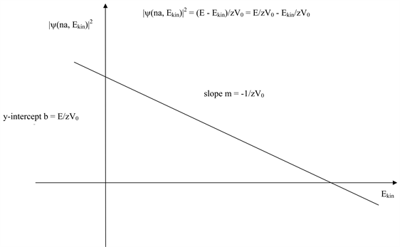
Figure 1. The material quantum probability density is drawn against the kinetic energy Ekin yielding a linear graph with the slope of −1/zV0 and an y-intercept of E/zV0.
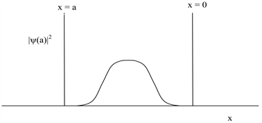
In the first case we assume E = Ekin, that means the total energy E is equal to the kinetic energy Ekin. As mentioned above, the probability distribution is zero at the Delta potential x = na, that means no material quantum is located at the Delta potential. Consequently, the material quantum is located not at the Delta potentials, but it is located between them due to the normalisation condition as shown in Figure 2(a). Consequently, the probability density betweent two adjacent Delta potentials is maximum, so the first case describes the state of lowest energy.
In the second case the kinetic energy Ekin is gradually reduced thus yielding , the probability density at the Delta potential x = na is increasing steadily and linearily as shown in Figure 2(b). So the probability density at the sites of Delta potentials x = 0, x = a and x = na is small, but not negligible any more, while the probability density betweent two adjacent Delta potential becomes smaller.
In the third case, the kinetic energy Ekin is further reduced, thus the probability density at the Delta potential x = na is further rising, so at the sites of Delta potential becomes significant, while the probability density between two adjacent Delta potentials is further reduced (Figure 2(c)).
In the fourth case, the kinetic energy Ekin is still decreasing and the probability density is still rising, until the probability density function x: becomes constant (Figure 2(d)). This case marks a turning point, because now the probability density at the sites of Delta potential becomes larger than the probability density betweent two adjacent Delta potentials (fifth case, see Figure 2(e)).
In the sixth case Ekin is equal to zero and so Ekin attains its minimum value, consequently reaches its maximum value E/zV0, while the probability density betweent two adjacent Delta potentials becomes minimum or even zero (sixth case, see Figure 2(f)). That means that the probability density at the sites of Delta potential is equal to E/zV0. In this situation, the material quantum is located at the Delta potentials (the sixth case describes the state of highest energy).
Although, in the third, fourth and fifth case (Figures 2(c)-(e)) a normalisation problem occurs: because the third, fourth and fifth case does not match with the normalisation condition . This can be very well observed in the fourth case (see Figure 2(d) and Figure 2(g)): the probability density function x: is constant and thereby delocalisated throughout the entire Delta potential array; that means it reaches theoretically from plus infinity to minus infinity. In order to comply with the normalisation condition, the probability density must become almost zero as it is shown in Figure 2(g). Although this is mathematically not forbidden, this does not make any physical sense. Consequently, while the first case (Figure 2(a)) is physically allowed and senseful (low energy) and while the sixth case (Figure 2(f)) is also physically
 (a)
(a)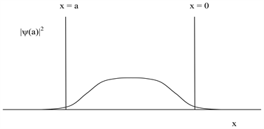 (b)
(b)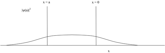 (c)
(c)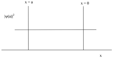 (d)
(d)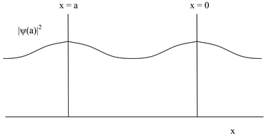 (e)
(e)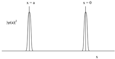 (f)
(f)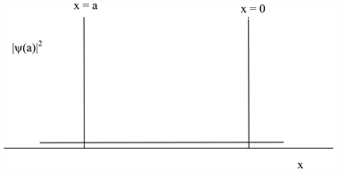 (g)
(g)
Figure 2. (a) The material quantum probability density distribution inside of an array of Delta potentials is shown; in the case of Ekin = E: the material quantum probability density distribution is zero at the site of any Delta potential , while the material quantum probability density distribution is maximal in the space between two adjacent Delta potentials . (b) In the case of Ekin decreasing and thus a little bit smaller than E: is small, but not zero at the sites of Delta potential, while is slightly decreasing between two adjacent Delta potentials. (c) In the case of Ekin further decreasing: is further increasing at the sites of Delta potential, while is further decreasing between two adjacent Delta potentials. (d) In the case of Ekin continues to decrease: is increasing at the sites of Delta potential, while continues to decrease between two adjacent Delta potentials, until is equal to and the material quantum probability density function x: becomes constant. (e) In the case of Ekin still continues decreasing: continues increasing at the sites of Delta potential, while continues decreasing between two adjacent Delta potentials, thus becomes larger than . (f) in the case of Ekin = 0: is equal to E/zV0 and thus maximal, while is equal to zero and thus minimal.
allowed and senseful (high energy), the fourth case is forbidden physically (medium energy), which is equivalent to the existence of an energy gap in a solid state lattice. But in case of quantized space and material quantum this energy gap makes the difference between light and mass: In the first case (if E = Ekin and thus is zero that means the material quantum is located between two adjacent Delta potentials (Figure 2(a))) then the material quantum is representing a “mass quantum”, while in the last case (if Ekin = 0 and thus is maximal that means the material quantum is located at the site of a Delta potential (Figure 2(f))) then the material quantum is representing a “light quantum” or photon.
One can compare the situation with the harmonic oscillator treated classically and by quantum mechanics (Figure 3) [25] . As shown in Figure 3, at the lowest energy level (so-called zero-point energy level), the probability distribution density is maximal at the center and almost zero at the side lines. This corresponds to the situation in Figure 2(a), where the probability distribution density is also maximum at the center (x = a/2) and minimum at the side lines (x = 0, a). Classically treated, the harmonic oscillator is resting and so pending at the center where it spends all its time, while it spends no time at the side lines. At higher energy the probability distribution density of the harmonic oscillator becomes lower or almost zero at the center and is increasing at the side lines (Figure 3). This corresponds to the situation in Figure 2(f), where the probability distribution density is minimum at the center (x = a/2) and maximum at the side lines (x = 0, a). Classically treated, the harmonic oscillator spends most of its time at the side lines (turing point with v = 0), while it spends the least of its time at the center (transition with maximal velocity).
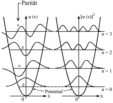
Figure 3. Harmonic oscillator treated quantum mechanically: at the lowest energy level (so-called zero-point energy level) the probability distribution density is maximal at the center and almost zero at the side line, while at higher energy the probability distribution density becomes lower or almost zero at the center and is increasing at the side line.
Consequently the situation of the material quantum between two adjacent Delta potentials (Figures 2(a)-(f)) can be interpreted as a vibration formally similar to a harmonic oscillator, but with a decisive difference: at the highest kinetic energy Ekin the probability distribution density of the material quantum is maximum at the center of the cubic space quantum and minimum at the Delta potentials located at the side lines of the cubic space quantum (Figure 2(a) and Figure 1: point of intersection between graph and axis of abscissae), while at the lowest kinetic energy Ekin the probability distribution density of the material quantum is minimum at the center of the cubic space quantum and maximum at the Delta potentials at the side lines of the cubic space quantum (Figure 2(f) and Figure 1: point of intersection between graph and axis of ordinates). In case of a harmonic oscillator it is quite vice versa: at low kinetic energy the probability distribution density is maximum at the center and minimum at the side lines as above discussed, while at high (kinetic) energy the probability distribution density is minimum at the center and maximum at the side lines (or to be more precisely: in the momentary state of maximum kinetic energy, is minimum at center and in the momentary state of maximum potential energy, is maximum at the side lines).
Eventually one can interpreted this as something similar to an inverse (harmonic) oscillator.
Optionally one can cited that Schrödinger Equation yields that the material quantum starts vibrating only after the insertion into a cubic space quantum confined by Delta potentials as described above. Before insertion into the cubic space quantum, no vibration occurs. So one could eventually assert that the material quantum becomes a string only by insertion into a cubic space quantum due to the presence of the equally spaced Delta potentials which makes the material quantum vibrating. Without any Delta potentials in its surrounding, the material quantum is nothing else as a non-significant zero-dimensional punctual material quantum without any physically relevant features or characteristics and totally lost in space, time and universe.
This could be vaguely and faintly similar to an oscillator featured by a Higgs potential as well as to the Higgs postulation citing that a particle mass arises only by interaction between a particle and the Higgs field.
3. Conclusions
In the attempt to find an unified field theory, it is an usual way to contrive a novel field whose covariant derivation yields a field strength tensor and thus a Lagrange density. But until now this approach has not succeeded.
This can be explained by an array of Delta potentials as the novel field as follows: A field or an array of Delta potentials cannot be covariently derived due to irregularities at the site of Delta potentials. But the Delta potentials are the relevant feature or characteristics of such a novel field, because elsewhere the potential is zero. This could eventually explain why until now no Lagrange function has been found by covariant derivation.
Another advantageous aspect of the theory of arrayed Delta potentials as the novel field is the formation of gravitation waves only in case of mass acceleration. It is well-recognized that resting or constantly moving mass objects without any acceleration does not produce any gravitation waves, while in case of acceleration gravitation waves are generated. This can be simply explained by the model of arrayed Delta potentials: In case of resting the mass quantum stay in their cubic space quantum and nothing happens. In the state of unaccelerated moving the mass quanta are migrating with a constant velocity v across the cubic space quantum, whereby at the site of the Delta potentials the mass quanta are scattered. The frequency f of the scattered wave is assumed to be linearily proportional to the mass quantum velocity v: f µ v. In a very simple case of two subsequently arranged Delta potentials, the migrating mass quanta (moving with constant velocity without any acceleration) are scatterd at the site of the first Delta potential generating a first scattering wave with the first frequency f, and at the site of the second Delta potential the migrating mass quanta (still moving with the same velocity) are also scattered generating the second scattering wave with the same frequency f. So it is imaginable that by the right choice of phase difference between both scattering waves, the two scattering waves totally destructively interfere with one another, thus nothing is left due to the completely destructive interference.
Now we consider the following case: the migrating mass quantum is accelerated thus at the site of the first Delta potential the mass quantum has a velocity of v1, and the mass quantum is scattered by the first Delta potential generating a first scattering wave with the first frequency f1 µ v1. In the meantime the mass quantum is accelerated. Thus at the site of the second Delta potential the mass quantum has the velocity v2. There the mass quantum is scattered again generating a second scattering wave with the frequency f2 µ v2. Now f2 > f1 due to v2 > v1 and f µ v. By this reason a complete destructive interference between both scattering waves is not possible any more because f2 is not equal to f1, but f2 is slightly larger than f1. Instead the superposition of the two scattering waves yields a beat with a modulation frequency . Exactly this beat is perceived as a gravitation wave with the frequency .
If the acceleration vanished, that means the acceleration becomes zero, the frequency of the beat also becomes zero and the gravitation wave disappears. This could explain why gravitation waves only occurs in case of acceleration and not in case of non-acceleration.
This simple model is valid only for one dimension. Eventually by time and space quantisation one can generalize this model to three dimensions.
Conflicts of Interest
The author declares no conflicts of interest regarding the publication of this paper.
Cite this paper
Wochnowski, C. (2019) A Very Simple Model Concerning the Unified Field Theory Basing on the Kronig-Penney-Model. Journal of High Energy Physics, Gravitation and Cosmology, 5, 941-952. https://doi.org/10.4236/jhepgc.2019.53050
References
- 1. Veneziano, G. (1968) Construction of a Crossing-Simmetric, Regge-Behaved Amplitude for Linearly Rising Trajectories. Il Nuovo Cimento A (1965-1970), 57, 190- 197. https://doi.org/10.1007/BF02824451
- 2. Galli, E. and Susskind, L. (1970) Structure of Hadrons. II. Nonplanar Diagrams. Physical Review D, 1, 1189. https://doi.org/10.1103/PhysRevD.1.1189
- 3. Susskind, L. (1970) Structure of Hadrons Implied by Duality. Physical Review D, 1, 1182. https://doi.org/10.1103/PhysRevD.1.1182
- 4. Galli, E. and Susskind, L. (1970) Structure of Hadrons. II. Nonplanar Diagrams. Physical Review D, 1, 1189. https://doi.org/10.1103/PhysRevD.1.1189
- 5. Susskind, L. (1969) Harmonic-Oscillator Analogy for the Veneziano Model. Physical Review Letters, 23, 545. https://doi.org/10.1103/PhysRevLett.23.545
- 6. Nambu, Y. (1969) Quark Model and the Factorization of the Veneziano Amplitude. Symmetries and Quark Models: Proceedings of the International Conference, Detroit, 18-20 June 1969, 269.
- 7. Nambu, Y. (1970) Lectures at the Copenhagen Summer Symposium.
- 8. Nambu, Y. (1970) Dual Model of Hadrons. EFI-70-07, 14.
- 9. Nielsen, H.B. (1969) An Almost Physical Interpretation of the Integrand of the n-Point Veneziano Model. Niels Bohr Institute, København.
- 10. Nielsen, H.B. (1970) Paper Presented at the XV International Conference on High Energy Physics. USSR, Kiev.
- 11. Polchinski, J. String Theory: Volume 1, an Introduction to the Bosonic String. Cambridge University Press, Cambridge.
- 12. Schwarz, J.H. (2000) Introduction to Superstring Theory. Lectures Presented at the St. Croix NATO Advanced Study Institute on Techniques and Concepts of High Energy Physics.
- 13. Witten, E. (1995) Some Problems of Strong and Weak Coupling. Univ. of Southern California, Los Angeles.
- 14. Witten, E. (1995) String Theory Dynamics in Various Dimensions. Nuclear Physics B, 443, 85. https://doi.org/10.1016/0550-3213(95)00158-O
- 15. Wilson, K. (1974) Confinement of Quarks. Physical Review D, 10, 2445. https://doi.org/10.1103/PhysRevD.10.2445
- 16. Penrose, R. (1971) Applications of Negative Dimensional Tensors. In: Welsh, D., Ed., Combinatorial Mathematics and Its Applications, Academic Press, New York, 221-244.
- 17. Penrose, R. (1971) Angular Momentum: An Approach to Combinatorial Space- Time. In: Bastin, T., Ed., Quantum Theory and Beyond, Cambridge University Press, Cambridge, 151-180.
- 18. Sen, A. (1982) Gravity as a Spin System. Physics Letters B, 119, 89-91. https://doi.org/10.1016/0370-2693(82)90250-7
- 19. Ashtekar, A. (1986) New Variables for Classical and Quantum Gravity. Physical Review Letters, 57, 2244. https://doi.org/10.1103/PhysRevLett.57.2244
- 20. Ashtekar, A. (1987) New Hamiltonian Formulation of General Relativity. Physical Review D, 36, 1587. https://doi.org/10.1103/PhysRevD.36.1587
- 21. Vaid, D. (2018) Connecting Loop Quantum Gravity and String Theory via Quantum Geometry. https://arxiv.org/abs/1711.05693
- 22. Kittel, C. (2002) Einführung in die Festkörperphysik. de Gruyter, Berlin.
- 23. Ibach, H. and Lüth, H. (2009) Festköperphysik. Springer, Berlin.
- 24. Bonc-Bruevic, V.L. and Kalasnikov, S.G. (1982) Halbleiterphysik. VEB Verlag, Berlin. Ashcroft, N.W. (1976) Solid State Physics. Brooks Cole, Monterey.
- 25. http://www.pci.tu-bs.de/aggericke/PC3/Kap_III/Oszillator.htm