Journal of High Energy Physics, Gravitation and Cosmology
Vol.03 No.04(2017), Article ID:80081,33 pages
10.4236/jhepgc.2017.34060
The Universe at Lattice-Fields
Giovanni Guido1, Gianluigi Filippelli2
1Department of Physics and Mathematics, High Scholl “C. Cavalleri” Parabiago, Milano, Italy
2Astronomic Observatory “Brera”, Milan, Italy

Copyright © 2017 by authors and Scientific Research Publishing Inc.
This work is licensed under the Creative Commons Attribution International License (CC BY 4.0).
http://creativecommons.org/licenses/by/4.0/


Received: August 3, 2017; Accepted: October 28, 2017; Published: October 31, 2017
ABSTRACT
We formulate the idea of a Universe crossing different evolving phases ( ) where in each phase one can define a basic field at lattice structure (Uk) increasing in mass (Universe-lattice). The mass creation in Uk has a double consequence for the equivalence “mass-space”: Increasing gravity (with varying metric) and increasing space (expansion). We demonstrate that each phase is at variable metric beginning by open metric and to follow a flat metric and after closed. Then we define the lattice-field of intersection between two lattice fields of base into universe and we analyse the universe in the Nucleosynthesis phase (intersection-lattice ) and in the that of recombination (intersection-lattice ). We show that the phase ( ) is built on the intersection of the lattices of the proton (Up) and electron (Ue) or . We show UH to be at variable metric (open in the past, flat in the present and closed in the future). Then, we explain some fundamental aspects of this universe UH: Hubble’s law by creating the mass-space in it, its age (13.82 million of Years) as time for reaching the flat metric phase and the value of critic density. In last we talk about dark universe lattice Ud, having hadronic nature, and calculating its spatial step (Dd) and its density in present phase of .
Keywords:
Space-Time, Lattice, Nucleosynthesis, Hydrogen Universe, Intrinsic Quantum Oscillator, Dark Matter, Dark Energy

1. Introduction
The Theory of Relativity establishes a deep physical connection between space, time and material objects (particles-fields): We cannot describe particles and their interactions without referring to space and time, and, at the other hand, the space and time haven’t a physical sense without objects (particles), in fact remember that a reference frame (RF) be built with material objects reciprocity at rest. Therefore, one could assert that if particles are to be considered like an objective reality, then also time and space, used for describe particles and their interactions, should be objectively considered as intrinsic “real characteristics” of the particles.
So like we state that the particles are in the Space-Time (ST) to same way we will say that the “Space-Time is into particles”. Remember that an elementary particle (i.e. electron) is seen in relativity theory like a point in Space-Time (ST) of any reference frame while in quantum theory it is seen like a field (Y). The characteristic of field in a particle is detected in his dual behavior (undulatory in Y and corpuscular in the quanta). If we associate a wave behavior to particle (you see the diffraction with electrons and photons) it is permissible to conjecture that “something” oscillates “inside” a particle: We talk about internal “clock” with proper frequency (ω0). Then it is permissible associating to particle also a wavelength (D0). If the frequency (ω0) generates the proper time (τ) of massive particle for symmetry it exists a wavelength (D0) that generates the “proper space” of the particle: We shall say that the “Space-Time is into particles”. We can conjecture that the mass is the physical expression of the proper frequency related to a particular elastic coupling between the oscillators of base field (X). One builds thus a massless scalar field (X) in whole Universe (XU) made by lattice of 1-dim. Chains of Quantum Oscillators (QuO) reciprocally coupled.
In (par. 2.1) we conjecture that the mass is given by a particular “transversal additional coupling” (called even “massive coupling”) between the oscillator chains of the base Ξ-Field.
This additional coupling builds a massive field (X) with lattice structure on the X-field, where is given a “Time Step” (τi) and a “Space Step” (Di) and on which it has empirical sense talking about Reference Frame (RF) associated with a massive particle (mi) with Compton wavelength (Di). In this way, the mass (mi) of each particle could be identified by a distinct and articulated structure of coupling of Quantum Oscillators (QuO) of the XU-field. We indicate this as “Structure Hypothesys” of massive particles (par. 3.1) in X-field. Moreover, it becomes possible to assign to a set of identical massive particles, with mass (mi) a field with lattice structure (
) which we will call “lattice-field” of universe or “universe-lattice”, denoted by Ui. The “universe field”
-field will be expressed by two components
relatives to base X-field and to the set of lattices Ui associated to the respective basic massive particles mi. Then, we note that when a massive particle is created concurrently to its (Space-Time)- lattice we are forced to add space (you see the Di) and time in universe (or to
) because itself is space and time. So, we show that the origin of the expansion of the universe is to be found in a sort of “creation of space” resulting to the “creation” of massive particles (
) in various universe-lattices Ui. Idem one can say about the cosmic time.
We make note that the universe expansion is detected to be a mutual spacing between galaxies; then, there is a physics equivalence between showing that this is caused by an increasing “quantity” of space interposed between them or that the expansion is a “stretching” of the space.
In (par. 3.2) we show that the mass meaning presented in our theory do no admits negative values of mass or do not exist antimatter associated to initially negative masses also if after these are transformed in positive particles by CPT-symmetry; this demonstrate that negative Lagrangians associated to antimatter exist no which can origin a repulsion between matter and antimatter, as instead it is proposed by some physicists (you see Villada) in opposition to General Relativity (RG). Then we show that la present theory is instead coherent with the Equivalence Principle (EP) and it proposes a relativistic cosmology.
In (par. 4.1) it is shown that in the Ui universe-lattice the Hubble law can be derived precisely by the “creation of space” resulting by the birth of (mi) massive particles in Ξ. See the universe expansion as space in increasing it is physically equivalent to reaffirm that the expansion is the expression of a particular property of the space different the one of the gravity.
In (par. 4.2) it is shown that a universe with “flat” metric exists only if there is a state of balance between gravity (originated by mass) and space (also originated by mass).
In (par. 5.1) we define the idea of “lattice field” present in the whole universe or Universe-lattice Ui, built on the particles of some type with mass mi. If number (n) of massive particles increases (increasing mass), that is (mi è nmi), it follows that Ui increasing in space to pass of time (time evolution). This balancing mass-space (you see par. 5.1) is achieved by each lattice Ui only at a certain moment of its evolution, where over time the Ui increases in mass (increasing number of particles) as well as in space. Thus Ui (par. 5.1) is a universe with a “variable metric”, going from a value of negative curvature (open universe for future reference) with accelerated expansion to one of positive curvature (closed universe) after going through an intermediate critic phase with a critic value of metric (flat universe). It is proved that the time (τc) to reach the critical phase is connected to the coupling gravitational constant (αi) of each Ui. In (par. 5.2) we define the universe-lattice UH like the “intersection” between the pair of universes-lattice (Up, Ue), because it is assumed (by the standard model), that our universe U is built on particulars set of base universe-lattice Ui, such as that of the electron (Ue) for leptons and that of the nucleon (Up) for the baryons (quarks).
Then, we consider that the hydrogen atom builds (through the intermediation of the photons, the quanta of the electromagnetic field) the intersection between
the two lattices or .
This allows to say that our universe is an “Hydrogen Universe”.
This aspect makes determine the factor (ks) which allows the “overlap” of the Compton wave lengths of two universe-lattice [(Up), (Ue)].
We obtain (in par. 5.3 as well) by simple calculations that the (τc) of (U)H is coincident (within the errors range) with the (τ) present age of our universe, defined only by astronomical observations (you see spatial telescope Planck). This leads us to believe that our universe is now in flat metric phase because it is near to the next critical phase of a universe with a variable metric.
Always in par. (5.4), it is noted that rc critical density of (U)(n,e), is greater than the one calculated in “nucleon masses” (rn)c and this detects the need of existence of a mass not visible that it bridges gap the difference between two density (missing mass). In par. (5.5) we analyze the phase of Nucleosynthesis built on the universe-lattice UN which is intersection of two lattices of hadrons. We make see that UN reach the value of critic density just in an antecedent time to that of the recombination. In par. (6.1) we build into UH a universe lattice of base Ud. We utilize the intersection-lattice between Ud and a Baryonic universe-lattice UB (you see ) for build the universe-lattice of dark mass UD, because we conjecture that the dark matter has a baryonic nature but interacting only gravitationally with the ordinary matter. We then calculate into UH the density of dark mass and we find a value next to one of critic density, so answering to question of missing mass.
2. The Mass
The Massive Coupling
Remember the world line representing the time succession of events in S’ (reference frame at rest with the particle) or proper time (τ) and the velocity of particle (4-velocity (ui)) which has a time component and a spatial. The time component of (ui) in RF at rest is [u4 = ic], which tells us that the succession of events in S' can be seen like a “movement in time” with imaginary velocity given by the constant (c). This characteristic is associated to any massive object, because when this takes to exist thus it will “move” in time. This uniform motion in time recalls once again the “clock”: so, it should exist every inside the particle-object a periodical “motion” which produces the motion in time. Then we will say about this as an internal clock with the proper frequency (ωo); it follows the correspondence . Therefore, it must exist a characteristic (X) of object which is connected with its motion in time, rather it is the generator of it. Follows so that this characteristic has to be connected to the proper time (τ) of the object ( ) and to satisfy at the same relations to which the (τ) and (t) satisfy:
(2.1)
where the time (t) is that of clock placed in other RF and (g) is the ratio of time dilation in the Lorentz transformations.
The new conception of “motion in time” allows also to understand the notion of the energy (E0) at rest: a massive object with motion in time has like an “energy of motion in time”. If the speed in time is (c), we can suppose that [E0 µ mc2] remembering the classical expression of kinetic energy. The logical sequence of correspondences between physical characteristics of particle is:
(2.2)
Therefore, it follows that . Conjecture then that the proper characteristic X, connected to the proper time (τ) of object, coincides just with the mass (m), thus putting that (X = m) or proper mass (m0). Thus if talking about mass or mass energy of a particle we talk about time of a clock that is inside them. Remembering the proper time (τ) it is
(2.3)
So even the (4-velocity (ui)); it follows the set of relations:
(2.4)
This last relation recalls the one of photon: . Following the quantum mechanics (see the photon):
(2.5)
If we associate a wave behavior to particle it is permissible associating to it also a wavelength (D0). If the frequency (ω0) generates the proper time (τ) of massive particle [τ = h/mc2], for symmetry it exists a wavelength (D0) that generates the “proper space” of the particle. Following De Broglie, we have:
(2.6)
We state that Dc = h/mc (the Compton wavelength) defines the spatial step of the proper space-time of massive particle.
Now, combining the equation of the relativistic energy with that of De Broglie and of Einstein, we have:
(2.7)
This last equation is the dispersion relation of waves described by Klein- Gordon equation:
(2.8)
As it is well known, the Klein-Gordon’s wave equation describes also a scalar field associated to massive particle with spin zero:
(2.9)
But there are also scalar field
with spin zero associated a no massive particles. Remember that an any scalar field
is physically equivalent to perturbation X propagating in “elastic medium” made by coupled oscillators elastically as in a system of beads with mass (M) connected through springs of elasticity constant (k) and length (L) [1] . You see the Figure 1:
If we have [(T = kL); (r= M/L) it follows
where (v) is velocity of propagation of an elastic perturbation (wave). The wave equation is:
(2.10)
We note the type of Equation (2.9) describes [1] also the oscillations in a set of pendulums coupled through springs (Figure 2):
In this system it’s [(ω0)2= g/l]. If we admit [l = (D0)], having [g = F/M] and [F ≡ T] it follows:
(2.11)
In elastic medium (X-field) it is [v2= T/r], while in reference frames at rest and in S-T 4-dim. it is ; therefore will be:
. By Equation (2.6) it follows:
(2.12)
It follows the Equation (2.5).
Following the relation (2.7) and Figure 2, we conjecture that the mass is the physical expression of the proper frequency related to a particular elastic coupling which is additional to the one already existing between the oscillators of

Figure 1. Field equivalent to set of beads with springs.

Figure 2. Set of pendulums coupled through springs.
massless scalar field (X). This “additional coupling” which produces the mass in a scalar field (X), it will be pointed out as “massive coupling”.
Therefore, we will associate a scalar field (X) to each massive particle havingan additional coupling (see T in Figure 2) compared to that of (X). The analogy with a system of elastically coupled pendulums moves us to associate a lattice-field ((Xi) to a particle-field mass (mi) where one can talk about space (Di) and time (τi).
The oscillation frequency ω0 of these “pendulums” when the “springs” (the oscillators of the field X) are not involved determines the mass value [m = (hω0/c2)].
The (Dc) the Compton wavelength is associated to proper oscillation (ω0) between the equation [Dω0 = c]. Then we can conjecture that the massive particle-field (X) is built by a “transversal coupling” (T0) between chains of oscillators of the scalar base field (X). We can represent in figurative way as it follows (Figure 3):
3. The Background Field of Universe
3.1. The Scalar Field of Universe (XU)
We note that in any lattice at massive coupling (see Figure 3) is possible to define a dimension spatial and time. It is just this way which pushes us to affirm that a massive particle carries with itself the Space-Time, see [(D), (τ)]. Then we could admit that it is possible define the S-T in any frame reference built between only with massive objects, because these carry the S-T with themselves. It follows that only massive particles introduce in Universe the dimension “Space- Time”. Besides, if any massive particle is built using the transversal additional coupling on X-scalar field, we may state that in universe there is a (XU) background field with structure scalar, in which an any massive particle is built by a particular structure of transversal couplings of quantum oscillators of X-field.
This presses us to assume that a massive particle is structure of articulated couplings between chains of oscillators of the X-scalar field of universe; we indi-

Figure 3. Massive field as lattice of “pendulums” with springs.
cate all this as “Structure Hypothesis” and we call (XU) as the “Scalar Field of Universe”.
The propagation of a particle into Universe is so the propagation in (XU)-field of a structure with “massive” coupling of quantum oscillators of X-scalar Field. Note that non massive (XU)-field do is not coincident with “the ether” because this cannot constitute a reference frame (RF). On the contrary a massive particle (massive scalar field) with transversal coupling introduces a local RF (S0) with a motion in the proper time (τ) and a spatial dimension (D0). Then we can consider the universe as a set (SU) of the local reference frames (S0), associated with massive particles. The symmetry group of the universe based on the lattices is the Poincare group. Now, we can build a whole RF for every galaxy as well as for clusters of galaxies until whole universe. The reference frame (RF) of each galaxy of the universe coincides with the “comovent RF” [2] defined by actual cosmology, to which a proper cosmic time (τc) is associated equivalent to the age of the universe. We could associate an only and unique field of base to each “comovent RF” in any galaxy: this will be a massive scalar field of fund which will indicate with (XG). So as we associated to single massive particle a reference frame at rest with a proper space and proper time, at same way we associated to whole galaxy an unique RF with proper ST (see the cosmic time).
Therefore, once more we will talk about Universe as “Universe Field” (XU) ≡ (XU, XG), of which the fundamental nature is the Space-Time. But we have not believe that (XU) is a sort of elastic ether pervading an absolute space, refuted by the theory of relativity, because the field (XU) is itself the cosmic space-time (you see the RF comovent) which an any observer of the universe represents and uses. We could also conjecture that the dark matter is in relation with (XU): [XU ó (XG) ó XD], where (XD) is the field of Dark Matter (you see the halos of dark matter around any galaxy). Because we asserted that a massive particle introduces in universe the dimensions of the space and time [(Dc), (τ)], we wonder if the expansion of universe is due to creation of massive particles which “add space” in universe: [mi ó(Di)]. To lattice of massive couplings that represents the massive particle (mi) we can associate a field (Xi) seen as a system of chains of quantum oscillators which couple in way transversal (massive coupling), with step (Di). We may so associate to the particle a field-lattice of chains of quantum oscillators. If a massive particle (mi) is represented by massive lattice in (XU)-scalar field, we can add to this lattice ulterior particles with same mass: we talk about “universe-lattice” of particles (Ui). If the number of massive particles (mi) is increasing we may hypothesize that (Ui) is increasing also in space: (Ui) should be so increasing in “mass-space”. Following the Standard Model and the structure hypothesis we could suppose that only the basic fermions (electron, for leptons, and proton, viewed like quarks (u) and (d), for baryons) can determine some processes of space-mass creation in the universe, because they are basic structures of couplings of the Quantum Oscillators. We take in consideration the fermions because for each chain of field-lattice with transversal step (Di), it is possible placing one only particle (one quantum).
All this allow us of conjecture that the creation of massive particle in U-Un- iverse could “creates” new space (see the Dc) and new “time” (see the cosmic time (τ)c) or adds space-time into universe. By this asserts we can conjecture that the expansion of universe (XU) could be the effect of a space increasing continually derived by Space creation in [(Xi) Ì (XU)].
As we will show after, the creation of mass-space can determine lattice-fields with variable metric. However, in this paper we not talk about sources of matter in the various universe-lattices, showing solely what happens in a universe with lattice-fields increasing in mass-space and with variable metric. Only in the section “conclusions” we will mention to a possible origin of matter into Universe that builds it with variable metric without to contradict the principle that the “Universe is all that is”. Besides we introduce the idea that the universe crosses in the course of time different evolving phases. Then, we so consider a U*-universe constituted by different universe-phases each of them built on specific universe-lattice (Ui)*. The last universe-phase (that in which we are living) started in time of recombination: (U*)rec.
3.2. Matter-Antimatter Symmetry in the Universe Lattices
The present theory of the “lattice shaped field” or “lattice-fields” is built on the hypothesis that the “mass” is the physical variable describing the additional “transversal” coupling between “chains” of quantum oscillators which represent a particle-field. In these systems (see par. 2.1) the “monotone mode” of oscillation is associated to the (ω0) proper frequency (see the Equation (2.7)) which indicates the mass. So the nature of the mass is that of being an oscillatory characteristic; note: an oscillation frequency is always positive. Not only, recalling the relations of [frequency ó clock] and [mass ó energy at rest], we have establish (par. 2.1) a relation between the energy at rest and energy of “motion in the time”: so in the reference frame at rest (S°) of a massive particle we cannot give an any physical meaning to the reverse motion in time. In any other reference frame (S) the particle will move in the time (in forward) and also it will move in the space of this reference frame (S). In relativity, if we reverse the time in an any relativistic equation the energy will be negative: there will be particles with negative energy which in the reference frames at rest (S°) will have negative mass or negative energy a rest. For what has already been said, in our theory we cannot have particles with mass negative. If instead we insist to admit hypothetical particles with negative energy, the reading experimental will give always particles with positive energy going forward in time but in spatial direction opposite (e.g. see about a system of an atom source (A) of particle massive and a detector atom (B)): for negative energies we will see B as transmitter and A as receiver and if the emitted particle has an electric charge then from B to A we will see a particle with opposite charge). In this way particles with negative energy exist no experimentally: this happens both in the special relativity that in general. In fact, the gravity admits as sources only masses with positive values. Also when one takes in consideration a platform in proper rotation and its curvature is negative, the mass of the platform is always positive.
Also more dangerous is the association negative energy ó antimatter. In literature some authors (see Villata in arXiv:1302.3515v1 [physics. gen-ph] 2013) take in consideration this aspect which, in my opinion, produces some problems in physics. In fact, in Villata the reversal of time in CPT transformation is associated to antimatter but this determines a Lagrangian LA opposite to that of matter LM. The emerging contradiction is the one of not associate a negative mass to reversal of time, because in this case (with m < 0, t ® −t) the Lagrangian result invariant [LA = LM], aspect in contrast with the result of Villata where it revers only the time: [LA = −LM]. The negative Lagrangian determines:
• [H = −p0 < 0]
• a gravitational field generated by antimatter which is indistinguishable by that generated by matter
• the possibility that a “local” CPT-transformation on the particles with negative Lagrangian and a local inversion of the time connected to the metric of the surrounding gravitational field determines repulsion with the surrounding matter
Following this road, Villata obtains that matter and antimatter are mutually repulsive and this should be the origin of the cosmic speed-up as well as the well-known universe expansion. The origin of this problematic aspect could be caused by two lacking considerations:
• The CPT-transformation operates in quantum systems and the charge electric is a variable correlated to wave function of particle but no correlated to the Space-Time of the reference frame from which an observer detects it.
• The mass and its gravitational field operate only in Space-Time “system” where we collocate the fields
We note that the antimatter in pair creation processes is always with positive energy: the coupling of two photons (positive energy) creates two particles with positive energy but with opposite charges. So in pair annihilation processes is an error to associate a negative value of mass to the positron, because matter and antimatter vanishing. Besides, two particles with positive energy have positive mass a rest and they determine a gravitational interaction to positive curvature: this result is in contrast with the Villata’s hypothesys that matter and antimatter repulse reciprocally.
As one knows, the positron has positive electric charge, see the conjugation operator (C), because a hypothetical particle whit negative energy (E < 0) going back in time (T) can be interpreted as a particle whit positive energy going in direction opposite (P) but with opposite electric charge (C). The conjugation of charge leads us to operate the CPT transformation when we speak of matteró antimatter. As it is know, the electric charge (±e) is correlated to the phase of the wave function of a particle because it is the generator of transformation U1 on the phase: [Q ó U1]. The gauge local invariance on the transformation of phase is guaranteed by photon which keeps the electric charge invariant in electromagnetic interaction. This shows that the electric charge is a variable relative to undulatory aspect of particle or to the oscillators of field (recall the field as a set of coupled quantum oscillators). In this way the CPT symmetry is a property typically of quantum systems or of systems with wave-particle duality. The antimatter is the transformed for CPT transformations of matter associated to solutions at negative energy of wave equation or to negative frequencies of the quantum oscillators of field. The CPT transformation as also the pair creation processes create particles always with positive energy (m > 0). All this leads us to admit that when we reverse the time the apparent negative energies are seen (thanks to CPT symmetry) as particles at positive energy but with electric charge opposite. The antimatter is the interpretation (the transformed) of the matter at apparent negative mass or negative frequencies. For overcome the problem of the presence of negative frequencies (or negative masses) it is need that the negative frequencies come “detected” without any reference to energy. Recall that in the oscillation theory we associate to the oscillation a rotation (see also the phase rotation). If the negative frequencies are associated to clockwise rotations of phase while that positives to anticlockwise rotations of phase (see Guido [3] ) and these rotations are associate to sign of electric charge, then only particles with negative electric charge or positive will exist but always with positive energy and mass. All this is possible only if a photon is able to detect the direction of phase rotation. In Guido ( [3] [4] ) this is showed. In this way we cannot associate negative value of mass to antimatter. Besides, the gravitational interaction do not perturbs the gauge invariance of electromagnetic interaction because it no causes variations to direction of phase rotation of wave function: the gravity do no transforms an electron in a positron. Nevertheless, the gravitational interaction is in turn a gauge invariant interaction: the graviton can cause some phase shifts (see interference phenomenon with neutrons in gravitational field) but, like photon, no changes the electric charge. Instead, the graviton acts on the tensorial fields which express the metric of S-T of reference frames (see the gravitational waves perturbing the S-T of “detectors”). In the gravitation the local gauge invariance on the metric is instead, the Equivalence Principle (EP) which not distinguish different values of mass (or so the signs ±) and so there is not any difference between positrons and electrons in free fall in earthling gravitational field. Any theory talking about repulsion between matter-antimatter should be in contrast to the EP. A cosmologic theory which explains the galactic acceleration through the matter-antimatter repulsion should be so in contrast with GR to the which any cosmologic theory is based. In this paper the mass express the additional coupling between chains of oscillators of a quantum field, building so a “lattice shaped field” or “massive lattice”. The (gik) tensor gives the metric of this lattice while the gravitational interaction between “lattices” is expressed by (Rik) Riemann’s tensor. Any gauge transformation on the wave function of particle (massive lattice) not perturbs the symmetry of local gauge of gravity or this not distinguish positrons and electrons. In final, our theory being built on the lattices of field is, therefore, coherent to EP and can solely express a relativistic cosmology.
4. Universe to Accretion of Mass-Space
4.1. The Accretion Law
In literature the universe’s expansion is regarded as the expansion of a spherical surface. We see, like observers, that the galaxies are immersed in a 3-dim space, “increasing” in volume, however, the cosmological principle imposes galaxies placed above a surface. If we add the time axis at every point of the universe by then a spherical surface 4-dim. is given. To increase a surface portion of a plan is necessary to increase the (X, Y) axes of a (DX, DY). The “expansion” of the spherical surface portion corresponds to add elementary steps (D) along the X and Y axes, which on the surface “spherical” 2-dim. become two meridians: [(X + DX), (Y + DY)]. Remember, indeed the expansion of a flat geometric figure in a computer: the program that performs the graphics operation increases the number of components “points” in Figure 4:
Note that to extend in way isotropic the surface in Figure 4, the mouse of PC points at point (A) and moves along the OA diagonal. This makes increase the number of points (one adds other points of space) into circle which increases so in surface. In an isotropic universe any local observer O puts himself at the

Figure 4. Expansion of spherical surface.

Figure 5. Isotropic movement of Galaxies.
center of a sphere 3-dim. with ray Ri and places on its surface the distant galaxies from O (Figure 5).
An observer sees galaxies move away radially in space (3-dim) but describes the isotropic expansion as dilatation of a 2-dim spherical surface, in which it placed itself into origin of the local spherical cap. Into an any Ui universe-lattice belonging to universe-phase increasing in space, the ray Ri of any local spherical cap (3-dim) would increase as . Where it can be , it follows [(Rn)i ≈ nDi]; it will be, omitting i-index:
(4.1)
where Sn varies with increasing Rn; then the index (n) will be a function of time: n ® n(t); we calculate the following derivatives:
(4.2)
where Vn is the velocity of recession of a galaxy placed on the spherical surface of ray Rn. For any observer an evolving universe (Ui) is described by means of an increasing time as [t = nτ], from which we obtain
We calculate the following derivative
(4.3)
and combining with the Equation (4.2) it follows
(4.4)
We will have
we obtain
(4.5)
So we obtain a constant velocity. This is achieved because we did not consider the “aspect” of space increasing or in any time (τ) between two any points it is added ulterior space steps (D): this causes larger distances to increase at even greater times than the smaller ones (see thermal expansion of metals). Then we’ll have that a spherical surface increase more than those with a smaller radius. Then we may conjecture . This because in time (τ0) other (n) steps (D) are added on surface S which pass from to . It follows:
(4.6)
with a proportionality [D0 = kD], [n = n0] and [c = D0/τ0]; we calculate
(4.7)
Computing
It follows
If we assume then it follows
(4.8)
finding again the Hubble’s law.
4.2. Mass-Space Balance
We avoid cosmological problems of difficult resolution if we restrict our attention to the individual Universes-lattices Ui.
We can admit that if the number of massive particles (mi) is increasing in a universe-lattice Ui with spatial step (Di), then there is more gravity in Ui; however, in Ui there will be even a space increasing with a consequent weakening of gravity, because to each particle with mass (mi) which is created we have associate a spatial step (Di): [mi óDi]. It derives that Ui is an increasing universe- Lattice or in expansion. Note that each Ui universe-lattice if increasing with mass-space could be at variable metric in relation of have more masses or more space: each Ui universe-lattice is at variable metric. We define the Universe as the set of all universes-lattices Ui.
We intuit, then, that during the accretion of the universe, any universe-phase it goes to cross, it is possible to have a time of its evolution where it could be there a just balancing between gravity and space. Remember a flat universe be consistent with the cosmological solution of general relativity that admits just a “equable balancing “ between kinetic energy (expansion) and potential energy (gravity). We note that even in the universe-lattice Ui with accretion of “space- mass” it’s possible to associate the kinetic energy (Kexp) to the creation of space because each galaxy moves away by others. Also, if the increase in mass is correlated with an increase of potential energy (more gravity) then the fair balance, for the general relativity, corresponds to a fair balance between mass and space in a flat universe.
There are distinct possibilities on balancing Space-Gravity:
1) The balancing Space-Gravity is an invariant of the universe, from its origins (see relativistic cosmology)
2) The balancing Space-Gravity is reached only at a particular time of cosmic evolution (see inflationary cosmology)
3) The balancing Space-Gravity is reached at a particular time (tk) of each k- phase of cosmic evolution (universe at more evolutionary phases)
We may think that the universe crossed different phases in time (see ), each built on a particular universe-lattice Uk with variable metric. We remember that in general relativity the T mass-energy tensor of the universe (defined as everything that is physically observable) is constant, so determining a constant metric in time.
We avoid cosmological problems of the whole universe if we restrict our attention to the individual Universes-lattices Ui of any . We may admit in that the individual lattice Ui can be described by variable metric because there is a flow of mass-energy between different lattices Uj, with . So we can suppose that into universe ( ), with increasing mass-energy, the mass-energy tensor T is variable. However, one would must explain the existence of something that “nurtures” the mass-space (or T) of each universe ( ). In a theory where “the mass is the source of both space both of gravity”, we highlight the following possibilities: the increase in the number of massive particles (and not) in the universe generates more gravity (increasing curvature ó metric variation), but also the space is increasing with a consequent weakening of gravity (decreasing curvature).
In case of variable metric it can believe, then, that during the increasing of the universe ( ), there is possible have a particular “moment” or “phase” in which the universe ( ) achieves a fair balance between gravity and space: “having so much gravity as much as space”.
A equal balancing between gravity (mass) and space will thus be expressed by the relation .
By this condition is obtained the escape velocity:
(4.9)
If we combine [2] with the Hubble law (note that with the speed of expansion of a sphere with ray R is equivalent to a speed of escape from a distant center R):
(4.10)
We obtain
(4.11)
From which we get easily
(4.12)
So we find the critical density, well-known in literature, of a flat universe ( ):
(4.13)
This relation is valid both in each universe-lattice Ui of any both in whole universe (in each of its evolving phases ( ) seen as overlap or intersection of
individual universes-lattices: .
We admit so a universe that crosses different evolving phases where each phase is built on a particular universe-lattice Uk with variable metric, passing from an open metric to a closed through the flat phase.
5. The Universe-Lattice
5.1. The Metric of the Universes-Lattices Ui
The relations identifying any “lattice universe”, with and Ui “increasing” in mass-space, are given by
(5.1)
The increase of massive particles (mi) in Ui implies an “increasing” space with ray Ri and spatial step given (Di) on the increase. The gravitational coupling constant (α) takes the value:
(5.2)
It’s also noted
(5.3)
The first lattice-universe Ui which has been originated in the first moments of the universe could be built on the value of the Planck mass
(5.4)
We denote with (Upl) the Planck’s lattice-universe. Instead for (mi < mpl) we have Ui universe-lattice in masse-space increasing (where is N = n2).
(5.5)
The value of the specific critical density of each specific Ui (with (n) is the number of “time” steps) will be given by
(5.6)
The critical density, as already said, represents the balancing Space-Gravity.
It notes that this balance is achieved in each Ui lattice only at a certain moment of its evolution, where at passing time the Universe lattice Ui is increasing in mass (at increase of number N of particles) as well as in space. In fact (see Equation (5.5)) the Ui universe reaches his critical density when the (n) number of time steps is such that occurs:
(5.7)
Thus it follows
(5.8)
We point out that
(5.9)
For (n < ni) Ui is an open lattice-universe. Instead for (n > ni)
(5.10)
Ui is a closed lattice-universe. By varying (n) we have the following development of density (you see Figure 6).
In this way Ui is a universe with a “variable metric” in the phase ( ), going from negative curvature (open universe for future reference) with accelerated expansion to one of positive curvature (closed universe) after to going cross an intermediate “critic” phase with a zero metric (flat universe). Now it is proved

Figure 6. Evolution of the density curves in lattices Ui.
that the time (τc) to reach the critical phase in ( ) is connected to the coupling gravitational constant (αi) of each Ui. The time τc (critical age) to reach the critical density will be given by
(5.11)
We find
(5.12)
As examples, consider the universe-lattice of the electron (Ue) and that of the proton (Up), finding the respective “critical” time
(5.13)
(5.14)
We compare the two lattice-universes; in the critical phase it is
(5.15)
As well as for the Equation (5.2) and Equation (5.7) we obtain
(5.16)
And therefore:
(5.17)
Expressing the mass through D
(5.18)
It follows
(5.19)
We place
(5.20)
where Sc is defined as “Compton’s Surface” of a particle. We will denote by [Se º (Sc)e, Sp º (Sc)p]. We will be then
(5.21)
We can have
(5.22)
where we introduce a (k) numerical constant related to the physical various arguments that take into consideration. Remember that (ni/nj) is a rational number because (ni, nj) are whole numbers, while the ratio (Di/Dj) cannot be irrational if (Di) and (Dj) are not commensurable; therefore the numerical constant (k) can be useful for make commensurable the ratio (Di/Dj). With constant (k); so it’s
(5.23)
Taking the square root we have:
(5.24)
It follows even
(5.25)
And therefore:
(5.26)
where
5.2. The (U)(p,e) Universe-Lattice
We wonder what surface (S) can represent this equality [S = neSp = npSe]. The surface [(ni)Sj] (see Equation (5.22)) can have physical meaning only in an universe-lattice U(i,j) which “contains” the two distinct lattices Ui and Uj. This can be achieved only in a universe-lattice intersection of the two universe lattices Ui and Uj:
(5.27)
We note that the real universe cannot be built on only type of particle (mi ® Ui), you see the standard model. Then, one must conjecture a universe-lattice intersection of the universe lattices Ui of base. In an any universe-lattice the spatial step is given by (Dc), therefore to build the universe-lattice U(i,j) as intersection of Ui and Uj, the respective spatial steps should penetrate an into the other. We distinguish two cases:
• if (Di) and (Dj) are geometrically “commensurable” then the intersection will be represented as “superposition” of their direct lattices;
• if (Di) and (Dj) are “incommensurable” then the intersection can be built by use of a “intermediary” field that constitutes a background field where the two respective lattices can be in “superposition”
Whatever be the case in consideration, however, we could assume that [(ni) Dj] is the ray R* of U* º U(i,j). The same will be for universe-lattice in the critical phase [(ni) Dj] ó . Noting that if [neSp = npSe = SU] for any U universe-lattice and if
By Equation (5.21) è [RU = (ne)1/2Dp]; however we set in U* º U(i,j):
We will then (see the Equation (5.26)):
(5.28)
where [ks = (k)−1]. Let us consider the intersection of the two universe-lattice Up and Ue
(5.29)
We will geometrically (you see Figure 7).
Note that the actual universe U consists mainly of protons and electrons or Hydrogen, then we could assume that U-universe is “built” on an universe (U)(p,e), intersection of the two lattices (Up, Ue ); because into Universe there not is only Hydrogen lattice, we assume: [U É (U)(p,e)]. Note that the UH could be one of some evolving phases ( ) of Universe: we talk of the “Hydrogen phase”. The beginning of this Universe-Phase is coincident with recombination time. We wonder, therefore, if the hydrogen atom builds (through the intermediation of the photons, the quanta of the electromagnetic field) the intersection between the two lattices or [(U)(p,e) = (U)(H)]. The UH will be said “Universe lattice at Hydrogen”. If we consider the diameter of a hydrogen atom, we can assert that along the diameter a bond between the proton and the “orbiting” electron is established.
The diameter is given by QuO-chain where the “oscillations” of three particles (proton, electron and photon) can be in “superposition”. In hydrogen atom the Compton wavelength of electron is (Dleg = De/αem), where αem is the constant of electromagnetic coupling or also known as the fine structure constant. It notes that Dleg is exactly the Bohr ray è [Dleg ≡DH].
We will say then that the action of the electromagnetic field (photon) “adapts” the Compton wavelength of the electron to the one of proton to allow the intersection of the two lattices. Then the fine structure constant is a constant of “electromagnetic adaptation” between two electric charge with different structure. The adaptation happens along the diameter: for obtain the superposition of two lattices (Up, Ue) the DH must be projected along the chain-diameter because the wavelength lp is projected along the chain diameter and an orbital electron is physically equivalent to an oscillating electron along diameter. Nevertheless, being electron and proton of different spatial “dimensions”, then it must make an adaptation in scale (a gauge transformation): we introduce a “gauge factor” derived by ratio of the two periods (τp,τe) or wave lengths, for adapting space dimensions between the representative quantum oscillators of particles (p,e). Remember that two oscillators in coupling phase need of adaptation: the coordination between two oscillators involves the reciprocal adaptions in periods and wave lengths. Into H-atom (intersection D) we will have to compare wave lengths of proton and bound electron; it is [(DH/lp) ≈ 104]. We need to compare the orbital ray of Hydrogen with the Compton’s wave length of proton. Note that the electron moves long the circumference while the proton long the diameter. Then, after having made the “gauge wavelength” [neDH(10−4)] or “scale reduction one must adapting the orbital movement of the electron with the proton oscillation along the diameter or adapting the circumference with diameter (you see the (2π) irrational value and remember èCirc/ray = 2π). Into intersection ) follows: [(2π)npDp = neDH(10−4)]. Where (np, ne) are two any whole numbers. Point out the [(np/ne]) = ks]:
(5.30)
thus it follows:
(5.31)
(ks) is so the ratio (DH/lp) scaled by (104) factor. We define (ks) as adapting ratio. The general relation is: [(ks) = γ(lx/ly)(10s)]. Where (s) is the exponential of the scale factor which makes (ks) Î [1, 10]; (γ) is a coefficient relative at geometric aspect. In this case it is: γ = (2π)−1. We will have in UH (see Equation (5.28)) that:
(5.32)
This relation is valid in a universe being “critical”. Then we could develop the following system of relations:
(5.33)
These relations could allow us of calculating the τc critical age of the universe UH. Since UH is the intersection of two universe-lattices with variable metric, we can also assert that it evolves from an expansive phase with open metric to a phase of contraction with closed metric but passing through a phase a flat metric. By restoring (see Equation (5.22)), the multiplicative constant we can express this in UH:
(5.34)
here the numerical constant (k) will be in connection with numerical constant (k), because UH is intersection of two lattices Up and Ue. This leads (see Equation 5.34 and Equation 5.32) to following relation
(5.35)
5.3. The Phase of Universe-Lattice
The Hydrogen phase is characterized by UH lattice. The (τc)*º (τc)H time to reach the critical density of the flat-universe will be derived from the system of relations (see Equation (5.33)):
(5.36)
(5.37)
Remembering that [ks » 4] and the relation between (nc)i and αi, it will be
(5.38)
Approximate values of the constants in the fifth decimal place, we get
(5.39)
We have got the “critical” time of the universe U*. It should be noted that this value is very close to the estimated value of the age of our universe processing transmitted data from the Planck space telescope. If our universe U is approximated by U* then the “critical” age would be very near (if not identical) to age τ of the universe U. The observations [5] give an age of the universe equal to
(5.40)
The data shows that the value of “coincides” with age found by spatial telescope “Planck” [6] . Therefore, by comparing of the two times , we could assert that our universe may be in a phase “critical” to flat metric, as is evidenced by the astronomical observations which shown really an universe with flat metric. By the critical time value (according to Equation (5.39)) a value of the Hubble’s constant H* is given:
(5.41)
The value is compared so to one experimental derived by observations [7] of remote galaxies through WAMP satellite, to which is given an universe old of and with critical density . Note by data that the value seems instead to be closer to the value [7] derived from the analysis of Cepheids (for nearby galaxies, the source “HST and N. Wright.”). If we connect the value of H to a past time, because derived from observations of remote galaxies (Hpass º H(remote gal) º HWAMP), or H to present time (Hpres º H(nearby galaxies) º HCeph), then it is clear that is: . By comparison of the two data (both the values of H and time τU) it is noted that the recession velocity in the past was higher. Having that it follows that the current universe is flat. This means that in the past the recession velocity would have been greater than that of the “present” (nearby galaxies). It is noted then that the variable trend of the metric, from open to flat, be manifested into galactic “red shift” with gradient greater than that linear of the flat metric having origin in our present.
5.4. Critical Density in ( )
In a universe with variable metric ( ) the transition from open metric to flat should obtained itself by diagram [5] “red Schift-galactic distance” a gradient greater for remote galaxies (Figure 8, curve 5) with respect to the linear (curve 3) provided for a universe in flat metric (next galaxies) (you see Figure 8).
However, (as shown in Figure 8) we see that the observations place more distant galaxies (curves (4,6) to those of an open universe metric (curves 5). This means that here it would be an additional acceleration to that provided in a universe with open metric (you see [5] ). Here we talk of accelerating expansion (aexp) of the Universe. Nevertheless, in this cosmologic model an explanation can be given on this acceleration: the increasing space in space (or space addition inside space) could cause a “pressure” (because one introduces quanta, you see the equivalence massó space) with consequent galactic acceleration. This induce to think that the space pressure could represent the “dark” energy. Now we calculate the critical density (rc)U* for the Universe U* in (t = τc)

Figure 7. Compton’s Surfaces in intersection lattice of Hydrogen.
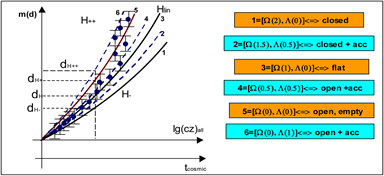
Figure 8. Reconstruction of the graphics of the figure report in [7] .
(5.42)
While the universe ray R* is:
(5.43)
It is evident that if it follows that R* » RU. By definition of the actual mass density of the universe derives the value of the total mass in number of protons. Nevertheless, we know the number of temporal steps needed to roach the critical phase in Up,e. because these are coincident with number of protons (np) in Up only that in U* the numbers of particles is in relation with spherical surface, therefore it will be
(5.44)
and
(5.45)
If we want to consider the baryons thus we add a numeric ratio b in Equation (5.44) or N = b(n2).
And so the baryonic density would be:
(5.46)
If we consider that the baryonic matter has been created in couple one obtains Np ®2Np:
(5.47)
The is, at less than factor of (10), next to experimental value of the density of visible matter:
In U* we observe that:
(5.48)
Note that:
(5.49)
Besides this:
(5.50)
From the Equation (5.31), we obtain that the protonic matter density is equivalent to critic density scaled by factor (10)4 around. In fact, if k = 4 we have (from Equation (5.50)):
(5.51)
Now we note that: the universe U contains all the universe lattices and all universe lattices reach their critical density at the same time. It thus follows that the universe U in “hydrogen phase” is flat together with all the universe lattices which compose it. However, remember that the Up universe is contained in the lattice UH (Up Ì UH) even if it (Up) reaches its critical density at the same time to UH (where UH is an “expanded universe” because the time step is that of the proton while the space step is that of the electron). Nevertheless, the density is higher in UH that in Up (should be on the contrary less for the “expansion”), this can mean that there must be other particular baryonic mass or non-baryonic mass which compensates the defect of density. This value tells us that there must be more mass in the universe to reach the critical density. This aspect opens the question of the missing mass: the astronomical observations however detect not radiative mass in the massive halos enveloping each galaxy (dark mass). Even at the dark mass it is associated a universe lattice Ud.
5.5. The Phase of Nucleosynthesis Universe-Lattice UN
Let us consider the intersection of the two universe-lattice Uα and Uπ
(5.52)
where (α) indicates the α-particle and (π) the neutral pion. Note that the UN could be a Universe-lattice representative of an evolving phases ( ) of Universe in which the first nucleus were formed: we talk of the “Nucleosynthesis phase” ( ). Note this phase is antecedent to that of recombination. The Nucleosynthesis phase is characterized by UN lattice. The (τc)* º (τc)N time to reach the critical density of the flat-universe derives from the system of relations (see Equation 5.33):
(5.53)
where (kN) is adapting ratio: [(ks) = γ(lx/ly)(10s)] where if [lx > ly] ó[s < 1]. The (η) is a coefficient connected to probability of interaction with nucleons: [ £ 1]. In our study [4] on the quarks we found that the geometric relation between the lp of pion and lα particle (α) is given by (j) “aureus” ratio (golden ratio). Let’s go find the (kN) adapting ratio:
(5.54)
We calculate (kN) and (αα), with (γ = j), where (j) is “aureus” ratio:
(5.55)
and
(5.56)
Now we can calculate the critical time (τc)N of universe-lattice UN of Universe phase ( ):
(5.57)
We have got the “critical” time of the universe . The critical density (omitting h) is:
(5.58)
So one can see that in the antecedent phase to that of recombination (Nucleosynthesis phase) the universe reached a flat metric (you see the literature) a few moments prior to the recombination.
6. Dark Matter
The Universe Lattice (Ud) of Dark Mass
Remember the U-universe composed by set of universe lattices Ui and by set of intersections of universe lattices ( ). We write: . We denote by (XU) the scalar field which contains the massive scalar fields (XO) of ordinary mass and (Xd) associated with the dark mass. We have: {(XU) É [(Xd), (XO)]}. Besides we think that the massive scalar fields of base in (XU) with commensurable Compton wave lengths can overlap one on the other if they come to cross a same space: so it is built a lattice Uu of interpenetrated lattices one inside the other ® . We will talk about a lattice of lattices Uu. In the representation of operators (a, a + ) when the number (ni ®¥) for any Ur universe-lattice the spectrum of Compton wave lengths can be a continuum, not only but the interpenetration of the lattices allows a continuous change of quanta between the varied lattices.
For n ®¥ we talk about Uu like a Universe-lattice in state of “fluid”. Now we define the Universe as [ ; , ]. The matter, both ordinary and dark, could present in this fluid state. Then, we could think that the universe-lattice of dark matter in particular phases can be in this fluid state because superposition of more universes-lattices of dark mass is {Ud}: . The massive scalar fields interact between them only gravitationally as it occurs in a fluid: a line of coupled quantum oscillators of field is like a line of flow into fluid. We think that this physical state is present in the galactic halos of dark mass. Thus we assume the dark matter like be a “static” fluid around each galaxy, this because in gravitational balancing. The indirect presence of the not radiative halos of matter enveloping each galaxy, induces us to admit that the representation of dark matter fluid can be that of a universe lattice of dark mass (Ud). Also the halos build a lattice of dark mass. We can admit that there are intersections of (Ud) with other lattices Ui, you see the galactic halos of dark mass enveloping galaxies of “hydrogen” (UH) or the influence of dark matter on the movement of stars around the galactic center. Because the whole matter in Universe is approximately baryonic matter (UB), we think that it is also intersection of (Ud) with lattices of baryonic matter (UB). To have a significant influence on the motion of stars, dark matter must be able to interact gravitationally and quantistically with elementary constituents of stars, that is with nucleons. This makes us think that the dark matter could have an hadronic nature, obviously electrically neutral, that is constituted by quark (u, d, s): we call this hypothesis as “hadronic hypothesis of dark matter”. Return to the “fluid idea”: we conjecture that particles of dark matter aggregates themselves into agglomerates of hadrons as it happens in the macromolecules. We will assume that:
(6.1)
where (B) is an any baryonic particle which couples to dark particle for originating the “hadronic macromolecules”. In intersection lattice UBd we will have:
(6.2)
and (kd) is a parameter yet to define. It follows, by Equation (5.33):
(6.3)
where [kd = (k)−1/2], you see the Equation (5.35) and (DB) = h(DB) with (h) coefficient connected to type of baryon. Nevertheless, we should think also that the two universes-lattices UH and Ud are in interpenetration or , because their gravitational interaction “adapts” field oscillators of any mass value. This could involve [RH = Rd] and also that [RH = Rd = RBd]; that is here we considering that the present ray of Universe is a “limit” ray for all universe-lattices in phase of expansion. In this case we will have:
(6.4)
If taking the neutrons (B ó n) as neutral baryonic matter, it follows that we will have the Fermi’s ray (DF) as ray of baryonic interaction, then (DB) = (DF) it is:
(6.5)
Nevertheless, the number of particles [N = n2]:
(6.6)
Recall the Equation (5.12), we obtain, in the case of the only lattice Ud:
(6.7)
where (md) is the mass of dark particle no coupled with matter: the mass associated to lattice Ud. Because we have supposed [RD = RH] then (md) is an average value of dark matter. We’ll have:
(6.8)
In (eV) we have:
(6.9)
This value is the “average mass” of dark matter in Ud if RU = Rd. To this value there are not known hadronic particles; the most next could be a “quark” component of a meson [4] . Nevertheless with a different value of (h) we could have greater value of (md). Now we can calculate the dark mass density of lattice UBd; it is :
(6.10)
We need find the (hkd) value. Speaking of hadrons, by value Equation 5.55 it follows:
(6.11)
If [kN = kBd] it will be in :
(6.12)
Now we can calculate the ratio between two density:
(6.13)
If [h =1] it follows:
With higher value of (h) one could have a density of dark matter greater. Now we search the value of Compton wavelenght of the particle of dark mass in intersection lattice ; we use the Equation (5.28):
(6.14)
Or
(6.15)
Calculating:
(6.16)
We determine the kBd value
(6.17)
It follows
(6.18)
The mass value less than of (h) is:
(6.19)
This is the value of dark mass that is in universe lattice of intersection UBd. Recalling the “hadronic hypothesis of dark matter”, we can think that this value is the mass value of hadron agglomerates of dark matter or “macromolecules” of dark matter.
7. Conclusions
It is evident in this paper that the idea of the universe structured in universes- lattice (Ui) of base and crossing different evolving phases ( ) at variable metric doesn't oppose to the actual model of universe. Each phase reach the flat metric, you see the Nucleosynthesis phase, where wave propagates in fluid nuclear are similar to that propagates in a fluid at flat metric, you see literature. Rather it tries to resolve some problem list leading and it opens the way toward new horizons on the birth and evolution of the universe. By this new approach we have tried to face the fundamental problem of the expansion of the universe, explaining it as “creation” of space in the Universe Field generated in turn by mass creation in the universe. Not only but it could explain also the galactic acceleration through the ulterior mass-space creation inside a preexistent mass-space where it could create an additional expansive pressure (you see the following analogy: you imagine a crowded place of people where in any point of it there is the materialization of “one” person; it should happens that this last will create a pressure around it toward the others). Our theory being built on the lattices of field at massive coupling is coherent with the EP and can solely express a relativistic cosmology. Besides correlating the mass to space this theory “completes” the GR: the mass acts on the space in “totus”, because the mass curves the space and produces it. Then, we will have that at “more mass” there is “more space” (see the Compton wave length). If we talk about [mass creation ó space creation] it is evident to propose the conjecture of a equivalence principle between mass and space. We could think so to new equivalence principle: the equivalence mass ó space. If the universe is the physical system of all lattices of field and these are increasing in the mass-space (and so increasing in “volume”.) then universe comes seen in expansion and in acceleration. This treatment doesn't put in the “shade”, at time being, the extended theories of gravity [8] , because the same EP mass-space push the physicists to manipulate the terms of the cosmologic equation of RG for explain the galactic acceleration. Say “more mass is equivalent to more space” in physical terms implicates varying the R tensor and T tensor in the cosmologic equation of GR. Instead the weak point of this “new” cosmology, should be the “mass creation”. This first article avoids the problem of the origin of the mass creation, by saying only that the universe observed by us could be built on some “lattice-fields” to “increasing mass” and spatial expansion, because some data obtained by this model coincide with those observed astronomically. Instead, in a second article in preparation, a relativistic cosmology with (L), not added ad hoc, is derived using properly the equivalence between “creation of mass-space” and “expansion”. In this article, we will hypothesize a state of “quantum vacuum” no built on the physical-mathematical aspect of the field constituted by a set of oscillators coupled in vacuum state; considering a quantum oscillator with semi-quanta and sub-oscillators (you see the idea of “IQuO” in Guido [3] [4] ) we can think to new state of vacuum built by an aggregation of “empty” sub-oscillators (a sort of “sub-quantum vacuum”); this state cannot be considered a state of field and so cannot be insert in the mass-energy tensor of the Universe. The matter (antimatter) could be originate by energy flowing from the “sub-quantum vacuum” to fields which component the universe. These aspects can be inserted in the equation cosmologic without (L) and to derive the complete cosmologic equation. We specify there that this procedure can be considered as an attempt of “extend” the gravity (you see bibl. [8] ); in this way this our theory could be considerate as belonging to the “extended theories of gravity”. Ulterior details obviously will be showed in the second article. Note the mass-space equivalence introduces a variable metric universe, that clarifies some cosmological problem list not still resolved by the Einstein’s relativistic cosmology:
・ The problem of Universe expansion problem described only mathematically and not physically by scale parameter a(t) associated to galactic distances
・ The Dark Mass problem
・ The unconvincing hypothesis that the universe became at flat metric during the inflation phase (change of metric in a “isolated” universe )
・ Expansive acceleration whose cause is a “mysterious” dark energy
Instead ours new explanatory thesis are remarkable:
・ the physical explanation of the expansion as the effect of creating “space” and no through “dark energy”
・ the creation of mass implies the creation of space or Space-Mass equivalence
・ the calculus of time age in the phase UH
・ the calculus of density
・ the variable metric caused by increasing mass
・ possible mass value of the dark matter and its density
This cosmologic model with mass increasing describes so an universe in which in actual phase (Hydrogen phase UH) is initially developed with variable open metric, it is reaching the flat phase after once of 14.82 billions of years from the BB and then it should pass to a metrics closed with prevalence of the gravitational force; this last will determine a deceleration of the expansion until the stop for after begin a phase of contraction. So it is admitted the possibility that to end of this phase of contraction there will is a “Big Crunch”. Nothing prohibit then another new Big Bang and therefore a new universe: we point out this possible universe as “Cyclical Universe”.
Acknowledgements
We would like to thank Dr. Christian Corda for his suggestions and advice in the preparation of the paper.
Cite this paper
Guido, G. and Filippelli, G. (2017) The Universe at Lattice-Fields. Journal of High Energy Physics, Gravitation and Cosmology, 3, 828-860. https://doi.org/10.4236/jhepgc.2017.34060
References
- 1. Crawford Jr. F.S. (1968) Waves. McGraw-Hill book Company, USA.
- 2. Zel’Dovich, Ya.B. and Novikov, I.D. (1983) Relativistic Astrophysics, Vol. 2—The Structure and Evolution of the Universe. The University of Chicago Press.
- 3. Guido, G. The Substructure of a Quantum Oscillator Field. arxiv.org/pdf/1208.0948.
- 4. Guido G. (2014) The Substructure of a Quantum Field-Oscillator. Hadronic Journal, 37, 83.
- 5. Perlmutter, S., et al. (1998) The Supernovae Cosmology Project (1998) Discovery of a Supernova Explosion at Half the Age of the Universe. Nature, 391, 51-54. https://doi.org/10.1038/34124
- 6. “Planck” Spatial Telescope NASA.
- 7. Perlmutter, S. (2003) Supernovae, Dark Energy, and the Accelerating Universe. Physics Today, (53):53[60,2003].
- 8. Corda, C. (2009) Interferometric Detection of Gravitational Waves: The Definitive Test for General Relativity. International Journal of Modern Physics D, 18, 2275. https://doi.org/10.1142/S0218271809015904