Theoretical Economics Letters
Vol.2 No.3(2012), Article ID:21508,3 pages DOI:10.4236/tel.2012.23062
Water Resource and Power Generation: An Alternative Formulation*
School of Economics and Finance, Victoria University of Wellington, Wellington, New Zealand
Email: Jack.Robles@vuw.ac.nz
Received March 6, 2012; revised April 8, 2012; accepted May 10, 2012
Keywords: Water Resource; Hydroelectricity; Cournot Competition; Closed Loop Equilibrium
ABSTRACT
Crampes and Moreaux [1] provide a two period model of competition between a hydrostation and a thermal station for the generation of electricity. We modify this model to make it more directly comparable with an infinite horizon model. The closed loop equilibrium is characterized.
1. Introduction
Crampes and Moreaux [1] (CM) provide a two period model of competition between a thermal station and a hydrostation for the production of electricity. CM’s analysis is both broad and illuminating. However, their model contains implicit assumptions which make it difficult to compare with an infinite horizon model. In this paper, we modify CM’s model to facilitate such comparisons, and solve for the closed loop equilibrium.
An appropriately written finite horizon model is essential to the understanding of infinite horizon models. Robles [2] analyzes an infinite horizon model and shows that one can characterize Markov Perfect Equilibria by finding the appropriate closed loop equilibrium to a one year finite horizon model.
A thermal station acts much like any firm. The hydrostation produces energy with (essentially) no variable cost. However, it’s output is constrained by the quantity of water in it’s reservoir. It can mitigate this constraint by passing water through time, but this ability as well is subject to constraint.
Our model has two main departures from CM’s: we allow for an over abundance of water as well as scarcity, and we allow water inflows in all periods rather than just the first. The second departure requires a third; our scarcity constraints are per period rather than global. We observe that in an infinite horizon model: no reservoir is large enough to prevent a firm from forcing it to overflow eventually, and water inflows must occur in more than one period. Consequently, an infinite horizon model must have all the constraints that we have added to the model. For the comparisons carried out in Robles (2009) to be meaningful, a finite horizon model must have these constraints as well. In addition, our departures from CM’s model: clarify the role of the various constraints, and allow the possibility of multiple equilibria.
2. Model
The model runs over two periods labelled . There is no discounting between periods. In each period, the thermal station produces
  and the hydrostation produces
  electricity. The per period (inverse) demand is denoted
 . The per period cost function for the thermal plant, denoted
 , is increasing and convex:

The thermal plant’s installed capacity is large enough that no constraint is imposed.
The hydrostation has no variable costs, but faces a number of constraints. Let  denote the stock of water available at the beginning of period
 . CM impose the resource constraint
 .
.
Like CM, we assume that  is set exogenously. However, we allow for an additional exogenous inflow of water between periods which we denote by
 . Hence,

Consequently, we need a resource constraint for each period. We also include a constraint on the hydrostation’s storage; the hydrostation must end the period with no more than  water. We assume that
  is sufficiently large that if
 , then the second period resource constraint can not bind in equilibrium. Further, we require that water is either used or passed to the future; there is no “spilling”. This implies the per period hydroconstraints 1 and 2:
 (1)
(1)
 (2)
(2)
Finally, we include a non-negativity constraint. For comparison CM: have no overflow constraints, and use a single resource constraint.
3. Equilibrium
We solve for the closed loop or subgame perfect equilibrium. In each period, firms set output. Demand,  , is downward sloping and such that each firm’s per period revenue function is concave in that firm’s own output. We denote the period
  revenue function for the hydrostation (resp. thermal station) by
  (resp.
 .)
.)
In each period the thermal plant acts to maximize profits within that period, . In each period
 , he satisfies
Here  is the multiplier on the thermal station’s period
  non-negativity constraint and the relevant complimentary slackness condition holds. Let
  denote the thermal station’s period
  reaction function.
Because of his constraints, the hydrostation’s optimal choice depends upon the stock of water . Let
. Let  denote the hydrostation’s optimal choice.
In the second period, the hydrostation’s problem is non-dynamic as well. However, he faces no variable costs, but must satisfy the hydro-constraints. The resulting first order condition is
 (3)
(3)
where ,
,  , and
, and  are (respectively) the multipliers on the period
  resource, overflow, and nonnegativity constraints.
Let  denote the solution to
If neither hydro-constraint binds in period 2, then  has no impact on output and
 . That is, the two firms behave like standard Cournot Duopolists.
In period 1, the hydrostation faces a dynamic problem, and acts to maximize . Of course
  enters directly into
 . However, it might also determine
  by setting
 . Hence, the hydrostation acts to satisfy the following first order condition:1
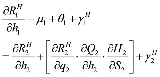 (4)
(4)
The LHSs of the hydrostation’s two first order conditions are analogous. However, the RHS of the period 1 first order condition might not be zero. Instead, it reflects the value of water in period 2. The first term on the RHS is the second period marginal revenue, holding  constant. The second piece is the strategic effect. It is never negative. It is strictly positive if
  and a second period hydro-constraint binds. In this case, an increase in
  leads to a decrease in
 . In response, the hydrostation will tend to move water from the first period to the second.
We turn now to a characterization of the various possible cases. First assume neither hydro-constraint binds in either period. Clearly the hydrostation sets 
at . Since this output does not depend upon
 , we have
  making the strategic term in Equation (4) zero. In addition, since the second period output is determined by
 , the remaining terms on the RHS sum to zero. Hence first period output is
 . That is, if neither hydro-constraint binds in either period, then we have period by period static Cournot competition. Our assumption that
  is large can now be formally stated as
 .
.
The preceding paragraph implies that the second period non-negativity constraint binds in equilibrium if and only if . This is as it should be, because the only other reason that a non-negativity constraint should bind is because of a desire to pass water to the future. However, in CM this constraint might bind because of a desire to use more than the entire resource of water in the first period. That is, CM’s second period non-negativity constraint might need to do the work that should be done by a first period resource constraint.
We consider next the possibility of a hydro-constraint binding in the first period. If this happens, and  , then the hydro station’s problem becomes static. That is, in each period t he acts as if to maximize period t profits. However, if
 , then the resource constraint might bind in the first period, but with
 . That is, the hydrostation would like to pass water backwards in time even though marginal revenue is negative in the first period. Of course, this requires that marginal revenue is even more negative in the second period.
We now consider the case in which a hydro-constraint binds in period 2, but no hydro-constraint binds in period 1. If the overflow constraint binds, then  and
and . If the resource constraint binds then
  and
and . In both cases, the two equations are redundant, and only determine the value of
 . However, if either of the hydro-constraints binds strictly, then
  and Equation (4)
nails down the exact values of  and
and .
.
We already established that if neither binds then
 . The possibility remains of a weakly binding second period hydro-constraint remains, in which case
  is undefined.
In equilibrium, the overflow constraint can’t bind weakly in the second period. Assume otherwise. If , then one can increase
  without decreasing
  and increase profits. If
 , then one can decrease
 , which increases profits by making the overflow constraint bind in the second period. On the other hand, the second period resource constraint can bind weakly. In this case, Equation (4) is not useful. However, when the resource constraint binds weakly, the equilibrium is easy to calculate;
 , and
, and .
.
Multiple equilibria are possible because whether the overflow constraint binds, or not, is determined endogenously by first period output. Since the two firms set output in each period simultaneously, there are circumstances where the hydrostation wants to force the overflow constraint to bind for some choices or , but not for others. That is, for some values of
  and
and , there are multiple equilibria.
We conclude with an example which illustrates how the water resource determines the equilibrium. Set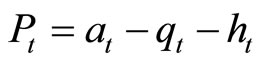 , a1 = 5, a2 = 8 and
 . Figure 1 illustrates the equilibrium outputs for the hydrostation as a function of the water supply. There are three general situations: water is scarce, water is abundant, and water
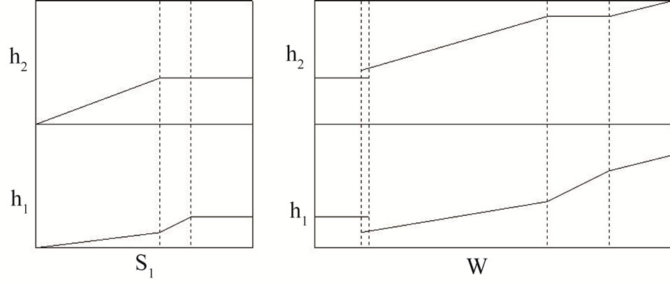
Figure 1. Example hydro outputs
is over abundant. The left hand box of Figure 1 graphs the transition from scarce to abundant; we set  and increase
  up from zero. From zero to the first dotted line, the second period resource constraint bindsand Equation (4) holds with
 . From the first to the second dotted line, the second period resource constraint binds weakly and
 . To the right of the second dotted line: no constraints bind,
  and
and .
.
The right hand box in Figure 1 graphs the transition from abundant to over abundant. We set , and increase
  from 0. To the first dotted line, the only equilibrium has
  and
and . At the first dotted line, there is sufficient water to support an equilibrium in which overflow constraint binds in the second period. Between the first two dotted lines, both these equilibria exist. At the second dotted line, the reward from forcing the overflow constraint to bind in the second period becomes too great, and the first equilibrium disappears. At the third dotted line,
  , which removes the strategic benefit from increasing
 . At the fourth dotted line, the marginal revenues are equal across the two periods, and so additional water is spread between them evenly.
REFERENCES
- C. Crampes and M. Moreaux, “Water Resource and Power Generation,” International Journal of Industrial Organization, Vol. 19, No. 6, 2001, pp. 975-997. doi:10.1016/S0167-7187(99)00052-1
- J. Robles, “Infinite Horizon Hydro Power Games,” Unpublished Manuscript, Victoria University, Wellington, 2009.
NOTES
*Thanks to Paul Calcott, and Vladimir Petkov.
1We are assuming for the moment, as CM do, that  and
and  exist. They may not.