Journal of Electromagnetic Analysis and Applications
Vol.07 No.03(2015), Article ID:54425,4 pages
10.4236/jemaa.2015.73007
A Method of Moment Approach in Solving Boundary Value Problems
Hilal M. El Misilmani1, Karim Y. Kabalan1, Mohamad Y. Abou-Shahine1, Mohammed Al-Husseini2
1Electrical and Computer Engineering Department, American University of Beirut, Beirut, Lebanon
2Beirut Research and Innovation Center, Lebanese Center for Studies and Research, Beirut, Lebanon
Email: hilal.elmisilmani@ieee.org, kabalan@aub.edu.lb, mya26@aub.edu.lb, husseini@ieee.org
Copyright © 2015 by authors and Scientific Research Publishing Inc.
This work is licensed under the Creative Commons Attribution International License (CC BY).
http://creativecommons.org/licenses/by/4.0/


Received 9 February 2015; accepted 2 March 2015; published 5 March 2015
ABSTRACT
Several available methods, known in literatures, are available for solving nth order differential equations and their complexities differ based on the accuracy of the solution. A successful method, known to researcher in the area of computational electromagnetic and called the Method of Moment (MoM) is found to have its way in this domain and can be used in solving boundary value problems where differential equations are resulting. A simplified version of this method is adopted in this paper to address this problem, and two differential equations examples are considered to clarify the approach and present the simplicity of the method. As illustrated in this paper, this approach can be introduced along with other methods, and can be considered as an attractive way to solve differential equations and other boundary value problems.
Keywords:
Boundary Value Problem, Differential Equations, Method of Moment, Galerkin Method, Weight Coefficient

1. Introduction
The design and analysis of electromagnetic devices and structures before the computer invention were largely depending on experimental procedures. With the development of computers and programming languages, researches began using them to solve the challenging electromagnetic problems that could not be solved analytically. This led to a burst of development in a new field called computational electromagnetics (CEM), for which powerful numerical analysis techniques, including the Method of Moment (MoM), have been developed in this area in the last 50 years [1] . Harrington in [2] describes the MoM as a simple numerical technique used to convert integro-differential equations into a linear system that can be solved numerically using a computer. When the order of the equation is small, MoM can analytically solve the problem in a general and very clear manner.
Although MoM has been studied in a large number of publications, it has been mainly a part of graduate courses on computational electromagnetics, or aimed to help professionals apply MoM in their field problems. In fact, it is infrequent to see a work on MoM addressed to undergraduate students to aid their understanding of this method, and help them apply it to solve problems they face in their undergraduate courses.
A large number of publications address the use of MoM in solving various problems. Djordjevic and Sarkar in [3] showed that the inner product involved in MoM is usually an integral, which is evaluated numerically by summing the integrand at certain discrete points. Newman in [4] has presented three simple examples on the use of MoM in electromagnetics. These examples deal with the input impedance of a short dipole, a plane wave scattering from a short dipole, and two coupled short dipoles. The use of MoM in electromagnetic field has been introduced by Serteller et al. in [5] . This is done by presenting examples and software program, and also by giving the curriculum needed to quickly learn the basic concepts of numerical solutions.
As mentioned earlier, the idea in this paper is to introduce the approach in a simple and straightforward manner to make it understandable to students taking basic course in differential equation. First, the method is defined and illustrated, a conversion into respective integral equation is determined, and then the unknown function is expanded into a sum of weighted basis functions, where the weight coefficients are to be found. The Galerkin method, which selects testing functions equal to the basis functions, is adopted. The problem then becomes a system of linear equations, which is solved analytically or numerically to find the needed weight coefficients.
2. Familiarizing Students with the Method of Moments
As the Method of Moments is based on expanding the unknown solution of the differential equation into known expansion and testing functions that satisfy the boundary value constraints, it is advisable to first introduce this approach in the solution. Accordingly, the sough of solution is expanded into a sum of known function, each satisfying the boundary conditions of the problem, with unknown coefficients to be determined by the solution. This determination is done with the help of testing function chosen similarly as the expansion function for the simplicity of the solution. The resulting equation is then converted into a linear system of equations by enforcing the boundary conditions at a number of points. This resulting linear system is then solved analytically for the unknown coefficients. This approach is very simple and quite interesting when applied to differential equation of order less than 3, but it will get more complicated for equations of higher order.
Accordingly, it is advisable to start with some basic mathematical techniques for reducing functional equations to matrix equations. A deterministic problem is considered, which will be solved by reducing it to a suitable matrix equation, and hence the solution could be found by matrix inversion.
Simple examples using linear spaces and operators are used. At first, it is recommended to introduce MoM and define some terms related to first order non-homogeneous differential equation. The choice of this equation is important only for better understanding of the solution.
A general nth order linear differential equation, defined over a domain D, has the form:
 (1)
(1)
In Equation (1), the coefficients  and
and  are known quantities, and
  is the function whose solution is to be determined. Equation (1) can be written in the form of an operator equation:
 (2)
(2)
where  is the operator equation, operating on
 , and given by:
 (3)
(3)
The solution of Equation (1) is based on defining the inner product , a scalar quantity valid over the domain of definition of
 , which is given by:
 (4)
(4)
Similarly, we define:
 (5)
(5)
The first step in calculating the integral, using Method of Moments, is to expand  into a sum of weighted basis functions
  in the domain of
 , as:
, as:
 (6)
(6)
Testing functions denoted  are defined in the range of
 . These testing functions are used for all values of
 . Using the inner product defined in (5), we obtain:
 (7)
(7)
Expanding Equation (7) over the values of m and , the following matrix equation is then obtained:
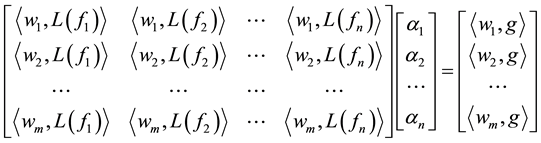 (8)
(8)
In a simpler form:
 (9)
(9)
and the solution for the unknown coefficients is then:
 (10)
(10)
In our calculations, the test function  is chosen to be equal to the basis function fn, which is known as Garlekin method. The determination of matrix
  is straightforward, and its inverse is easy to obtain either analytically or numerically. Once this is done, the
  coefficients are obtained, and the solution for f is found.
It is good to note here that choosing the appropriate basis/test function is necessary to get fast to the accurate solution.
2.1. Example 1
Considering the following second order differential equation defined by:
 (11)
(11)
defined over the domain  with the following boundary conditions
 . Starting by choosing the basis function, let us choose:
 (12)
(12)
It is clear from Equation (12) that the chosen basis function meets the boundary conditions and can be considered as a solution to the problem. Substituting Equation (12) into Equation (6), the left-hand side elements of Equation (7), which are the elements of the matrix , are found to be:
 (13)
(13)
In the same manner, we compute the elements of the matrix , defined in Equation (7), which are found to be:
 (14)
(14)
Then, we start by choosing , for which
  in
in  and
and , hence
 ,
,  ,
,  , and
, and  is given by:
 (15)
(15)
It is clear from Equation (15), that the function  does not meet the original differential equation defined in (11). Accordingly, we need to increase the value of N.
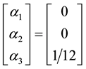
Let , and calculating the values of
 ,
,  and
and :
:
 (16)
(16)
Hence,  could be calculated as:
 (17)
(17)
Finally, calculating :
:
 (18)
(18)
The function  given in Equation (18) meets the boundary conditions defined in Equation (11), and accordingly it is the correct solution of the problem.
2.2. Example 2
Considering the following second order differential equation defined by:
 (19)
(19)
defined over the domain  with the following boundary conditions
 . Starting by choosing the basis function, it was noted that the basis function used in example 1 could also be used here:
 (20)
(20)
The chosen basis functions meet the boundary conditions and can be considered as a solution to the problem.  is calculated as in Example 1, since the same basis function is used, and it is given by:
 (21)
(21)
In the same manner, we compute the elements of the matrix , defined in Equation (7), which are found to be:
 (22)
(22)
Then, we start by choosing  for which
 . Accordingly,
  ,
,  ,
,  , and
, and  is given by:
 (23)
(23)
It is clear from Equation (23), that the function  does not meet the original differential equation defined in Equation (19). Accordingly, we need to increase the value of N.
Let , and calculating the values of
 , and
, and :
:
 (24)
(24)
Hence,  could be calculated as:
 (25)
(25)
Finally, calculating :
:
 (26)
(26)
The function  given in Equation (26) meets the boundary conditions defined in Equation (19), and accordingly it is the correct solution of the problem.
3. Conclusion
As demonstrated, MoM approach could be easily used to solve mathematical problems and equations. It can be easily employed by undergraduate students. According to the type of the equation, the solution of the Moment Method will vary to accommodate for the change in the given problem.
References
- Gibson, W.C. (2008) The Method of Moments in Electromagnetics. Chapman & Hall/CRC, Taylor & Francis Group, UK.
- Harrington, R.F. (1968) Field Computation by Moment Methods. Krieger Publishing Co., Inc., Huntington.
- Djordjevic, A.R. and Sarkar, T.K. (1987) A Theorem on the Moment Methods. IEEE Transactions on Antennas and Propagation, 35, 353-355. http://dx.doi.org/10.1109/TAP.1987.1144097
- Newman, E.H. (1998) Simple Examples of the Method of Moments in Electromagnetics. IEEE Transactions on Education, 31, 193-200. http://dx.doi.org/10.1109/13.2311
- Serteller, N.F.O., Ak, A.G., Kocyigit, G. and Akinci, T.C. (2011) Experimental Study of Moment Method for Undergraduates in Electromagnetic. Journal of Electronics and Electrical Engineering, 3, 115-118.