International Journal of Communications, Network and System Sciences
Vol.10 No.10(2017), Article ID:79843,11 pages
10.4236/ijcns.2017.1010013
A Markov Based Performance Analysis of Handover and Load Balancing in HetNets
Baoling Zhang, Weijie Qi, Jie Zhang
Department of Electronic and Electrical Engineering, The University of Sheffield, Sheffield, United Kingdom

Copyright © 2017 by authors and Scientific Research Publishing Inc.
This work is licensed under the Creative Commons Attribution International License (CC BY 4.0).
http://creativecommons.org/licenses/by/4.0/


Received: September 25, 2017; Accepted: October 22, 2017; Published: October 25, 2017
ABSTRACT
LTE heterogeneous networks (HetNets) is becoming a popular topic since it was first developed in 3GPP Release 10. HetNets has the advantage to assemble various cell networks and enhance users’ Quality of Service (QoS) within the system. However, its development is still constrained by two main issues: 1) Load imbalance caused by different transmission powers for various tiers, and 2) The unbalanced transmission power may also increase unnecessary handover rate. In order to solve the first issue, Cell range expansion (CRE) can be applied in the system, which will benefit lower-tier cell during user association phase; CRE, Hysteresis Margin (HM) and Time-to-Trigger (TTT) will be utilized to bound UE within lower tier network of HetNets and therefore solve the second issue. On the other hand, the relationship of these parameters may be complicated and even reduce QoS if they are chosen incorrectly. This paper will evaluate the advantage and disadvantage of all three parameters and propose a Markov Chain Process (MCP) based method to find optimal HM, CRE and TTT values. And then, the simulation is taken and the optimal combination for our scenario is obtained to be 1 dB, 6 dB and 60 ms respectively. First contribution of this paper is to map the HetNets handover process into MCP and all the phases of handover can be calculated and analysed in probability way, so that further prediction and simulation can be realised. Second contribution is to establish a mathematical method to model the relationship of HM, CRE and TTT in HetNets, therefore the coordination of these three important parameters is achieved to obtain system optimization.
Keywords:
Heterogeneous Networks (HetNets), Markov Chain Process (MC), Cell Range Expansion (CRE), Hysteresis Margin (HM) and Time-to-Trigger (TTT)

1. Introduction
In 3GPP Release 10 [1] , the Heterogeneous Networks (HetNets) were first applied and deployed as an LTE standard, in [2] , the 3GPP also introduced low- power and small-range radio based stations, such as pico and femto cells, these low-cost small cells access points that support fewer users compared to macro cells [3] . The adoption of these low-power nodes (LPN) allows the HetNets to contain more than one tier. The benefit of HetNets is obvious, such network make sure the mobility and is more convenient for user equipments (UE) to access. Due to the shorter distance between the UE and the network, the weakness of signal strength caused by path loss gets improved. Another advantage of HetNets is that the data transfer rate increased significantly because of the improving spectrum reuse efficiency [4] . However, HetNets also face several challenges due to its unique structure.
First issue is load imbalance caused by different transmission powers for various tiers. Due to structure of HetNets, UEs within the network may receive signals not only from same tier but also higher tiers. Since UEs prefer to choose signal with higher receiving power to obtain a better user quality of service (QoS), they may stick to higher tier cells and refuse to offload to lower tier cell. As a result, HetNets cannot operate efficiently higher tier cell that is overloaded while lower tier cell is of no use [5] . The second issue is handover problem, as afore mentioned, different transmit power in different tiers may cause frequent handover, among which, unnecessary handover occupied a considerable proportion. The system throughput will severe affected by the unnecessary handover.
In order to solve the first issue, the 3GPP first introduced the Cell Range Expansion (CRE) in release 10, this parameter can be considered as a virtual bias that added to the actual UE received power part to help UE with the association decision, the CRE is a practical power control technique in 3GPP standardization [6] . In a multi-tier network, most UEs are served by the macro cell because of its higher transmitting power and wider coverage area, compared with the macro cell, the transmitting power of small cell is much lower, typically, the transmitting power of macro and small cell is 40 Watts and 0.24 Watts [7] . As a consequence, if traditional user association is adopted, most UEs will be allocated to the macro cell, which may lead to a macro cell overload and much worse QoS experience. With the utilization of CRE, the UEs’ small cell receiving power strength is added by a CRE bias, which forces the UEs more likely to offload to small cells. This virtual bias limited the macro cell load and obviously stabilizes the UE when it travels around the cell edges, at the same time, the ping-pong handover probability is also reduced, which increased the network capacity [8] . However, the CRE only focuses on the load balancing issue without taking interference issues into consideration, meanwhile, the CRE will also change the UEs’ handover position due to the coverage change by the small cells.
The second issues can be solved by reasonable selecting different HM values to control the Handover Rate (HOR). As introduced in the previous part, the utilization of CRE will cause great impact in handover procedures. The deterministic of CRE is normally based on the cell load and network system performance, HOR is not considered when the CRE is chosen. It is introduced another virtual bias which is called handover Hysteresis Margin (HM) [9] [10] , to control the Received Signal Strength (RSS) during the UE association process. The HM is a constant variable which add to the serving cell RSS part, a handover decision will be made if the following condition is satisfied: 1) The target cell signal strength is larger than the sum of HM and serving cell signal strength, and 2) Condition 1 is satisfied for TTT time, where, the TTT is Time-to-Trigger which represent the time interval that handover condition is fulfilled [11] . Both HM and CRE are virtual bias added to networks, but the directivity of these two parameters is different. A good combination of HM and CRE can not only increase the system throughput but also reduce the HOR.
This paper is organized as follows, in section two, a brief introduction of HetNets system model is included [12] , then the detailed Markov Chain Process and its transition probability matrix is derived. In our previous work [13] , we only focus on the optimization of CRE but the relationship of other two parameters, HM and TTT, are not considered. In section of this paper, the simulation including further analysis of HM, CRE and TTT, which all take effects in the HetNets Handover process is taken according to our proposed method; and then the optimal values for three parameters in HetNets can be achieved.
2. System Model and Methodology
2.1. System Model
Figure 1 displayed the system model which is used in this paper, as we can see from that, a single macro to small cell scenario is adopted here. The cell radius of macro cell is set to be 1 kilometer, the total simulation area is set to be a 2 by 2 square kilometers square field. From the figure we can see that, a small cell is placed at a distance of D from the macro cell, for any UE inside the coverage, three parameters are assigned for it, with respect to the distance to the macro cell Dm, the distance to the small cell Ds, and an initial moving speed v.
With the set up of the aforementioned three parameters, the mobility model of the UE can be determined. We consider that each UE has its initial location information, moving speed and moving direction associating to the current
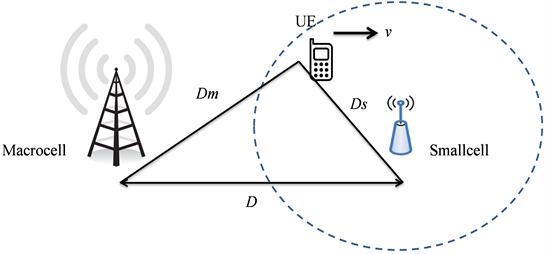
Figure 1. Two-tier HetNets System Model.
serving cell from time 1, which is represented by TTI 1. The current serving cell at TTI 1 is decided by the Receive Signal Strength (RSS) from different cells RSSm and RSSs. After TTI 1, the UEs will start to move as its assigned mobility model until TTI reaches 100. Due to the change of locations, UE’s distance to macro cell (Dm) and small cell (Ds) will change accordingly. When the UE move to the small cell boundary and the RSS of the serving and target cell represented by RSSS and RSST satisfy Equation (1) for TTT time a handover will happen.
(1)
Due to HetNets scenario applied in this paper, two different pathloss model is adopted for different tier UEs. The pathloss model for macro cell UE can be expressed as Equation (1). The distance d is in kilometres.
(2)
The distance d is in kilometres, the δM,t,k can be understanding as the pathloss of k UE at time slot t with macro cell M. In a HetNet scenario [14] , the pathloss for small cell and macro cell should be different, the pathloss model for small cell is shown as follows.
(3)
where the S inside the subscript represent the cell type is small cell. Then, we define the included angle θ as the angle of UE and small cell, the distance between macro cell and small cell is expressed as D which is shown in Figure 2. Following the cosine law, the relationship of Dm and Ds can be calculated as:
(4)
Based on Equation (2) and Equation (3) the RSSi,t,k of a certain UE allocated to a certain cell at each time slot can be calculated.
(5)

Figure 2. Markov Chain.
The Signal to Interference and Noise Ratio (SINR) can be derived from Equation (5), which is shown as follows.
(6)
In Equation (6), the numerator represents the receiving signal strength which is affected by variables i, t and k. Similarly, the interference is the summation of surrounding cells signal strength and expressed by the first part of denominator. While, the second part σ2 is the thermal noise.
2.2. Methodology
We applied the same Markov model from our previous work [13] . However, we take a further step and focus on analysing the relationship among CRE, HM and TTT and their effects on UE handover rate. Firstly, we apply Discrete Time Marokov Chain to model handover process so that all UEs’ association can be represented by Markov States. TTT is divided into several TTIs, and each TTI is defined as one step in MCP. For each step, UEs will follow their mobility model and generate a new distance relationship to nearby cells, so as the transfer matrix and status vector. According to TTT’s definition, UE will not initiate handover process unless its SINR is below the predefined threshold during whole TTT. As a result, M states are considered as the status where UE is link to macro cell, and S states are considered as the status where UE is link to small cell. Similarly, I and I’ states represent that UE is undergoing handover process (either from macro to small cell or small to macro cell). Finally, this handover process loop can be transferred into MCP, which is displayed as Figure 2.
In order to achieve the optimization values for HetNets, probability formula should be obtained from this MCP. Consider a UE’s initial state is M1, which represents that it is link to a macro cell right now. Its probability of moving to next state M2 is PM(x), meanwhile, its probability of moving back to itself is 1- PM(x). The same rule applies for all M states until Mn transfer to I1, which means that handover process is initiated. Within I states, it has 100% chance to move to next I state till handover process is finished and UE has been reallocated to small cell, which is in S1 state. The rules for S and I’ are the same for M and I states, so that the whole MCP loop is established. One important property for I and I’ states is that traffic signals play the dominant part to guarantee the handover process during these phases. Consequently, UE can barely receive information signal during handover states and too many handover phases will dramatically reduce the UE’s QoS.
Since we have understood all the states’ physical meanings, we may be able to establish transfer probability formula, which is PM(x) and PS(x) shown in Figure 2 (x is the number of TTI). In MCP, it represents the chance to continue checking handover status. As long as UE receives signals from both macro cell and small cell, it will have the probability moving to next state till handover process. Therefore, we define our MCP transfer probability as follows: Consider a small cell UE stays in S state, it will receive signals not only from macro cell (RSSM,x,k) but also from small cell (RSSS,x,k). These two signal powers will compete to transfer UE from S states to I’ states. When RSSM,x,k is the greater one, it will lead to the situation that UE has the intention to initiate handover process and reluctant to stay in small cell network. The situation will be opposite if RSSS,x,k is the larger one. At this time, HM bias, α, and CRE bias, β, will increase the weight of RSSS,x,k and constrain UE from moving back to the macro cell, which is shown in Equation (8). In Equation (7), however, they may play the opposite roles because CRE has another function to offload UEs from macro cell to small one.
The transfer probability formulas are expressed as below:
(7)
(8)
Transfer Matrix T can be obtained after the MC process and its transit probability is defined, then, the model of UEs’ handover process affecting by HM and CRE is established. Table 1 listed the transfer probability used in our simulation, it is a 4-state transfer matrix. After the set up of probability transfer matrix, the state probability vector V at x-th step can be calculated as Equation (9).

Table 1. Markov Transfer Matrix (T).
(9)
In Equation (9), the V1 is the probability of UE’s initial state, which is expressed as 1 in the vector. For example, if a macro cell UE is in the state M1 in time 1, then its initial probability vector will be expressed as [1, 0, 0, ..., 0]. With the TTI increases, the UE is moving, which will cause the probability Pmx and Psx changing in the Markov Transfer Matrix (T), according to Equation (9), the vector V will also change. As a result, the vector for any UE at any step x can be calculated, so that the HOR in each state will be obtained.
3. Performance Evaluation
In this section, simulation is taken to analyse the CRE, HM and TTT under different combination, the simulated parameters are summarized in Table 2 (all the simulations are taken by the MATLAB).
Figure 3 and Figure 4 show how handover rates react to CRE and HM with TTT = 40 ms. Generally speaking, it can be concluded that both CRE and HM will reduce handover rate as they grow. However, their influence degree may differ in many aspects. Firstly, the effect of CRE decreases rapidly and can be neglected when it reaches 9 dB, where handover rate stands still. While HM’s effect on handover rate keeps increasing and achieve the limitation when HM reaches 7 dB. Secondly, the starting and ending point of CRE and HM is different. HM can reduce handover rate from 9% to almost 0% while CRE can only make it to around 3%. All these phenomena display the superiority of HM in handover control, and the reason may be obtained from MCP probability formula and physical meanings of two parameters. HM’s main purpose is to delay the handover process and bound the UEs to their original serving cells, which including both macro cell and small cell. CRE, on the other hand, has another function to offload the UEs from macro cell to small cell so that decent HetNets
Table 2. List of Simulation Parameters.

Figure 3. Handover Rate vs. CRE.

Figure 4. Handover Rate vs. HM.
network efficiency can be maintained. As a result, CRE and HM may take opposite effects on handover control when UEs try to handover from macro cell to small cell. It also explains why handover rate will still remain 3% no matter what CRE value the network takes. However, HM’s effect on increasing total throughput is limited due to its lack of offloading effect in HetNets network. Its rapid effect of handover control also restricts that HM bias may not reach a large value. Therefore, an optimal combination of CRE and HM value is required for HetNets network.
Figure 5 shows how handover rate changes with CRE Bias for different TTT values. It can be observed that in four curves, handover rate will decrease with CRE, which follows our prediction by Equation (8). It is because that CRE virtually increases coverage of small cells and therefore restrains UEs’ handover from small cell to macro cell. With the growth of TTT, the initial handover rate drops dramatically, it suggests that increasing TTT will also benefit controlling handover rate. The ending point for each curve, however, increases slightly as TTT increases. This phenomenon is triggered by the increasing weight of β in
Equation (7), CRE will help to offload UEs from macro cell to small cell. As TTT’s effect on handover drops, CRE may lead a small growth of handover rate for I states in Figure 2.
Figure 6 introduces how handover rate changes with HM Bias for different TTT values. It shows that TTT has a significant effect in handover rate control, which follows the prediction of MCP as well. It can be reflected from two aspects: initial point and reaching-zero bias. When TTT = 40 ms, handover rate initial point is up to 18%, after which drops rapidly below 2% when TTT is set to 100ms. Besides that, HM’s reaching-zero point is also further limited as TTT increases, which is only 2 dB when TTT is 100ms. In other words, with selected TTT value, we may mitigate HM$’s side effect on system total throughput.
By analysing the relationship among CRE, HM and TTT, TTT is set to be 60 ms, which meets our predefined mobility model. Then, the combination of CRE and HM is simulated by optimizing system total throughput and Figure 7 is generated. According to Figure 7, 1 dB and 6 dB will be the optimal value for HM and CRE in this scenario.

Figure 5. Handover Rate vs. CRE under different TTT.
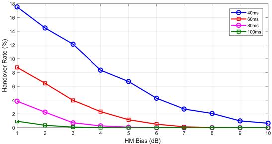
Figure 6. Handover Rate vs. HM under different TTT.

Figure 7. System Total Throughput vs. CRE and HM.
4. Conclusion
This paper proposes a Markov Chain Based Process to model HetNets system and analyses three main parameters during HetNets UEs offloading and handover―HM, CRE and TTT. This paper also establishes a mathematical method to model the relationship of HM, CRE and TTT in HetNets, therefore the coordination of these three important parameters is achieved to obtain system optimization. Finally, the optimal combination of HM and CRE for system performance is generated by our proposed MCP model, which is 1 dB and 6 dB respectively. However, the mobility model in our current work is not practical yet because we assume all the UEs’ velocity remains still during the whole TTT. In our future work, we will focus on establishing a more realistic mobility model and also take further study on how the velocity changing affects HetNets Handover.
Acknowledgements
This work was partly funded by the European Union’s Horizon 2020 research and innovation programme under grant agreement No. 734798.
Cite this paper
Zhang, B.L., Qi, W.J. and Zhang, J. (2017) A Markov Based Performance Analysis of Handover and Load Balancing in HetNets. Int. J. Communications, Network and System Sciences, 10, 223-233. https://doi.org/10.4236/ijcns.2017.1010013
References
- 1. Bjerke, B.A. (2011) LTE-Advanced and the Evolution of LTE deployments. IEEE Wireless Communications, 18, 4-5. https://doi.org/10.1109/MWC.2011.6056684
- 2. 3GPP (2012) TS22.220: Service Requirements for Home Node B (HNB) and Home eNode B (HeNB), Rel-11.
- 3. Zahir, T., Arshad, K., Nakata, A. and Moessner, K. (2013) Interference Management in Femtocells. IEEE Communications Surveys & Tutorials, 15, 293-311. https://doi.org/10.1109/SURV.2012.020212.00101
- 4. Lopez-Perez, D., Guvenc, I., De la Roche, G., Kountouris, M., Quek, T.Q. and Zhang, J. (2011) Enhanced Intercell Interference Coordination Challenges in Heterogeneous Networks. IEEE Wireless Communications, 18, 22-30. https://doi.org/10.1109/MWC.2011.5876497
- 5. Oh, J. and Han, Y. (2012) Cell Selection for Range Expansion with Almost Blank Subframe in Heterogeneous Networks. In Personal Indoor and Mobile Radio Communications (PIMRC), 2012 IEEE 23rd International Symposium on IEEE, 9-12 September 2012, Sydney, NSW, Australia, 653-657. https://doi.org/10.1109/PIMRC.2012.6362865
- 6. Okino, K., Nakayama, T., Yamazaki, C., Sato, H. and Kusano, Y. (2011) Pico Cell Range Expansion with Interference Mitigation toward LTE-Advanced Heterogeneous Networks. In Communications Workshops (ICC), 2011 IEEE International Conference on IEEE, June 2011, Kyoto, Japan, 1-5.
- 7. Krishnan, K.R. and Luss, H. (2011) Power Selection for Maximizing SINR in Femtocells for Specified SINR in Macrocell. In Wireless Communications and Networking Conference (WCNC), 2011 IEEE, 28-31 March 2011, Cancun, Quintana Roo, Mexico, 563-568. https://doi.org/10.1109/WCNC.2011.5779224
- 8. Andrews, J.G., Singh, S., Ye, Q., Lin, X. and Dhillon, H.S. (2014) An Overview of Load Balancing in HetNets: Old Myths and Open Problems. IEEE Wireless Communications, 21, 18-25. https://doi.org/10.1109/MWC.2014.6812287
- 9. Chu, X., López-Pérez, D., Yang, Y. and Gunnarsson, F. (2013) Heterogeneous Cellular Networks: Theory, Simulation and Deployment. Cambridge University Press, Cambridge. https://doi.org/10.1017/CBO9781139149709
- 10. Ray, R.P. and Tang, L. (2015) Hysteresis Margin and Load Balancing for Handover in Heterogeneous Network. International Journal of Future Computer and Communication, 4, 231. https://doi.org/10.7763/IJFCC.2015.V4.391
- 11. Kim, J., Lee, G. and In, H.P. (2014) Adaptive Time-to-Trigger Scheme for Optimizing LTE Handover. IEEE Wireless Communications, 7, 35-44. https://doi.org/10.14257/ijca.2014.7.4.04
- 12. Guidolin, F., Pappalardo, I., Zanella, A. and Zorzi, M. (2014) A Markov-Based Framework for Handover Optimization in HetNets. In Ad Hoc Networking Workshop (MED-HOC-NET), 2014 13th Annual Mediterranean IEEE, 2-4 June 2014, Piran, Slovenia, 134-139. https://doi.org/10.1109/MedHocNet.2014.6849115
- 13. Qi, W., Zhang,B. and Zhang, J. (2017) A Markov Based Cell Range Expansion Optimization in Two-tier HetNets System. International Journal of Engineering Technology, Management and Applied Sciences, 5, 17-25.
- 14. 3GPP (2013) TR 36.842: Study on Small Cell Enhancements for E-UTRA and E-UTRAN; Higher Layer Aspects, Rel-12.