Int'l J. of Communications, Network and System Sciences
Vol.4 No.1(2011), Article ID:3691,7 pages DOI:10.4236/ijcns.2011.41002
Adaptation in Stochastic Dynamic Systems —Survey and New Results I
School of Mathematics and Information Technology, Ulyanovsk State University, Ulyanovsk, Russia
E-mail: kentvsem@gmail.com
Received December 16, 2010; revised December 30, 2010; accepted January 4, 2011
Keywords: linear stochastic systems, parameter estimation, model identification, change point detection, learning and adaptive control
Abstract
This paper surveys the field of adaptation mechanism design for uncertainty parameter estimation as it has developed over the last four decades. The adaptation mechanism under consideration generally serves two tightly coupled functions: model identification and change point detection. After a brief introduction, the paper discusses the generalized principles of adaptation based both on the engineering and statistical literature. The stochastic multiinput multioutput (MIMO) system under consideration is mathematically described and the problem statement is given, followed by a definition of the active adaptation principle. The distinctive property of the principle as compared with the Minimum Prediction Error approach is outlined, and a plan for a more detailed exposition to be provided in forthcoming papers is given.
1. Introduction
In mathematical theory of data processing and control systems, the problem of overcoming a’priory uncertainty has a long history. As from the first principles of automatic optimizing control systems by Draper and Li [1], the first approaches to designing such systems by Kalman [2], and from the fundamental works on dual control by Feldbaum [3-6], it has been the focus of attention for many professionals, giving rise a host of publications in journals, conference proceedings and books [7], and thus determining the front line research in developing a theory and design of systems with the highest capabilities. The solution to this problem is naturally and closely associated with the concept of adaptivity.
As can be seen from the available literature, in an adaptive system the current information is percepted, analyzed, and used for the intentional change of the system. Thus, the adaptivity is realized here as the triune:
1) Classification of data percepted by modes of operation: the nominal mode or one of faulty modes; the corresponding block can be called Classifier.
2) Identification of the process model and/or measurement model launched when the faulty mode point is detected; the corresponding block is naturally to call Identifier.
3) System modification after the identification stopped with the new estimates for model parameters when the nominal mode point is detected; the corresponding block can be called Modifier.
These functions are not always broken into the three separate processes; in fact however, they are considered inherent to any adaptive system. Sometimes, identification is not separate from modification, and then no difference is made between these two processes. Such one-in-two process of changing the system is called, after Tsypkin [8], adaptation and the corresponding block adaptor (Figure 1), whereas making decision concerning modes of operation is sometimes called (for short) control over the system mode of operation. This term can imply emphasis on solving one of two (or both) subtasks: change detection and change point detection where “change” means switching from one mode of system operation to another. To equip the system with adaptivity, the crucial tasks to be solved effectively are the quickest change point detection and the unbiased estimation of the data source parameters, whose new unknown values may result from the change.
The quickest change point detection is of great importance for many applications and has extensive references
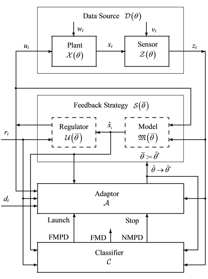
Figure 1. The generalized block-diagram of an adaptive system. FMPD—Faulty Mode Point Detected; NMPD— Nominal Mode Point Detected; FMD—Faulty Mode Detected. Legend: —external “reference” signal;
 — external “desired” signal;
 —uncertainty parameter;
  —suboptimal estimated parameter on which Feedback is based;
 —current estimated parameter;
 —final value of
  resulting from identification.
(e.g. [9] and many others). Parameter identification methods have also become the topic of a large body of research. However, little attention is still being given to the study of bias in parameter estimates. The bias in , the final result of identification, with respect to the true value
  of the uncertainty parameter
  is the most difficult to cope with when based on the incomplete noisy observations over a closed-loop stochastic control [10,11]. As this takes place, the existence of bias is not so annoying as its dependence on (unknown) experimental conditions [12].
2. Generalized Principles of Adaptation
The comprehensive and systematic analysis of existing system adaptation methods shows that design methodologies of adaptive filtering (state estimation) and stochastic control can be grouped into five large categories as follows.
2.1. Bayesian Adaptive Model (BAM)
The whole vector space of unknown model parameters is, firstly, partitioned and secondly, approximated by a set of design vectors. Based on each of those vectors, the optimal system is built, and the conditional (a’posteriori) probability density for each design vector is calculated to be used as a weighting factor for the system output. The approximation for the optimal estimate is computed as the weighted mean of outputs over the set of designed systems (Figure 2).
2.2 Extended Adaptive Model (EAM)
The state variable vector is augmented with the constant subvector of unknown parameters. Formed in this fashion, the extended model state equation is used as the basis for the optimal system design (Figure 3).

Figure 2. Bayesian (partitioned) Adaptive Model (BAM) principle: —a’posteriori probability densities,
 . (The small square-wise blocks denote multiplication.)
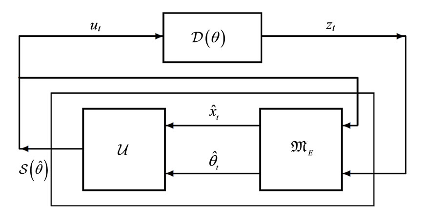
Figure 3. Extended (state based) Adaptive Model (EAM) principle: —extended model
  state vector.
2.3. Analytical Relations Based Adaptive Model (AAM)
The unknown parameters of the optimal system are expressed analytically or computationally through statistics of one or more chosen processes within the suboptimal system structure. These statistics are calculated through time averaging over a single sample representing the ensemble of samples for the chosen process. The analytical relations are then solved for the unknown parameters of the optimal system (Figure 4).
2.4. Performance Index Based Adaptive Model (PIAM)
In PIAM, the specifications are given in terms of the residual between an explicit reference signal and a model (predicted) signal. The model parameters are adjusted so that the model output would be close to that of real system taken as the reference. The mutual proximity of these outputs is taken as a performance index (a functional) to be minimized (Figure 5). Mininum seeking methods are designed to provide convergence of the adaptive model parameters to the values minimizing the performance index. It means that PIAM principle provides a closed loop identification scheme, i. e. the scheme with the feedback in performance index. The approach unites many methods: Minimum Prediction Error (MPE) method, Least Squares method, Maximum Likelihood method and many others [7].
2.5. Characteristic Matching Adaptive Model (CMAM)
An indirect and simplified performance index is intro-
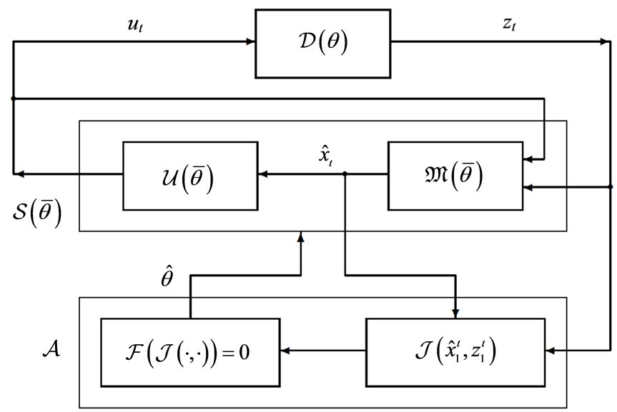
Figure 4. Analytical (optimality equation based) Adaptive Model (AAM) principle: —a statistic obtained from the sample
 ;
; —the model optimality equation.
duced instead of the original design performance index. Usually, it is defined as a deflection of a theoretical value of the inner system process characteristic from the corresponding actual value. The adaptation mechanism is designed to minimize this deflection (Figure 6). One possible technique for that is introducing a fictitious noise into adaptive model equations [13,14].
3. Dynamic System and Problem Statement
Consider a linear time-invariant state-space stochastic MIMO control system
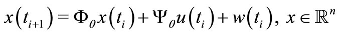 (1)
(1)
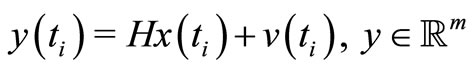 (2)
(2)
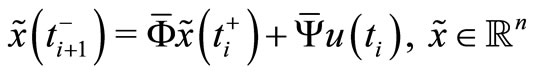 (3)
(3)
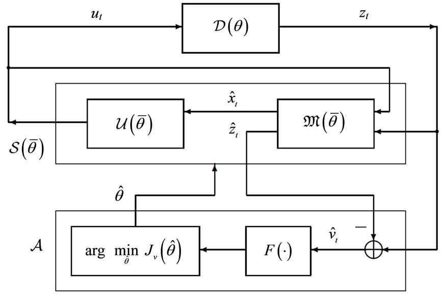
Figure 5. Performance Index based Adaptive Model (PIAM) principle: —an even loss function;
 —model performance index.
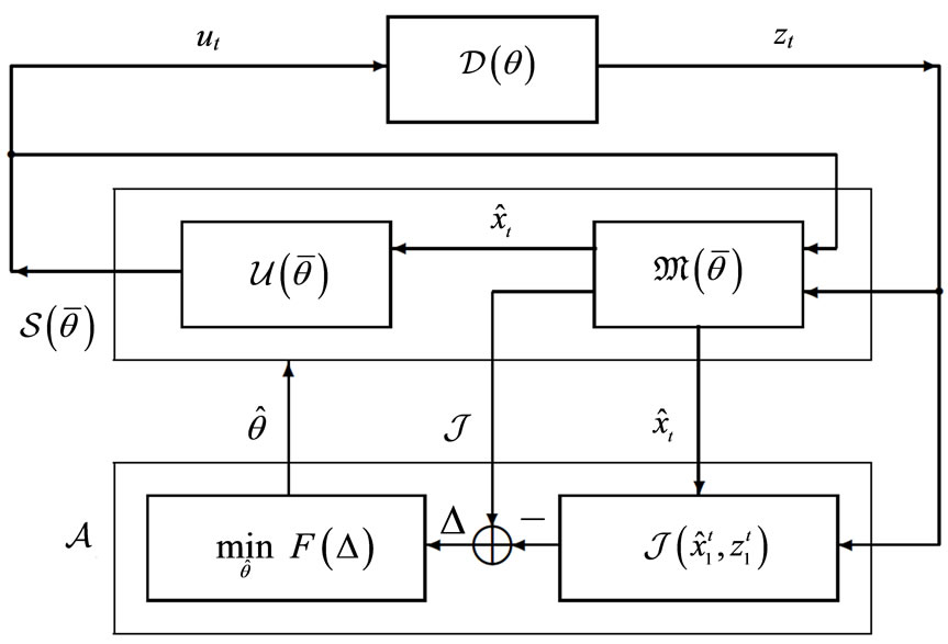
Figure 6. Characteristic Matching based Adaptive Model (CMAM) principle: —theoretical (predited) value of a characteristic;
 —experimental (virtual) value of the characteristic;
 —an even function of residual
 .
.
 (4)
(4)
 (5)
(5)
where , composed of a plant P, equation (1), a sensor S, equation (2), and a feedback controller FC, equations (3)-(5), realizing Feedback Strategy
  as shown in Figure 1.
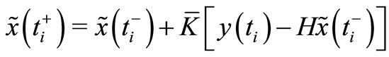
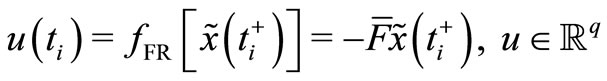
According to the separation theorem, FC is composed of a feedback filter FF, equations (3)-(4), cascaded with a feedback regulator FR, equation (5). Based on the Kalman theory, FF is the one-step predictor, equation (3), coupled with the estimator, equation (4). Note that in signal processing expositions, the process  in equation (1) is called the useful signal, the process
  in equation (2) the observation signal and
  the observation noise. In our case, the available data are complemented by control input
 , and so the observation data are
  at every instant
 .
.
The main assumptions are quite standard as follows. The random initial state  is given at some
  with
with  where
where  denotes the expectation of Euclidean norm
 ;
;  and
and  are zero-mean mutually orthogonal wide-sense stationary orthogonal processes such that
 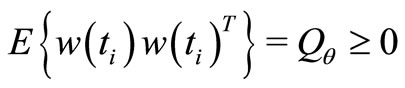 and
and 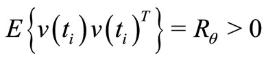 for all
  with
with  orthogonal to
  and
and  for all
 ;
;  given as a function
  of
of  is wide-sense stationary and
 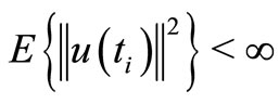 for all
 .
.
As we summarize the specific (but not restrictive) theoretical assumptions, we have the following:
A1 An infinitely long sample of observations  is a realization of a stochastic process on a probability space
  where the measure
  on the space
  is such that a form of ergodicity holds. For the purposes of this paper, it is sufficient to require the ergodicity in the mean for the inner processes of the system that are supposed to be wide-sense stationary. According to [15], the ergodicity theorem for wide-sense stationary processes states that the sample mean computed on increasing finite segments
  of the data will converge in quadratic means (q.m.) to the exact mean given in terms of
 .
.
A2 Plant equation (1) and sensor equation (2) are given by the standard observable model, SOM.
A3 Four matrices in the system description, namely the state transition matrix , actuator matrix
 , and noise covariances
  and
and  in the equations (1)-(2) depend on an uncertainty
  -component vector
 , as they are marked by the subscript
 . Each particular value of
  specifies a mode.
Remark 1 The resulting parameterization of ,
,  ,
,  and
and  by
by  has been suppressed for simplicity of notation. For the same reason, henceforth we shall write
 ,
,  ,
,  and
and  without subscript
 .
.
A4 The charts of the atlas covering the parameter manifold  constitute either a finite, countable or a continuous set. Thus the system itself can operate in several modes (finitely or infinitely many).
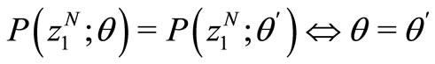
A5  constitutes an identifiable SOM parameterization [7], i.e., for all
  and all
 , we have
A6 The system is designed to operate with a minimum expected control cost
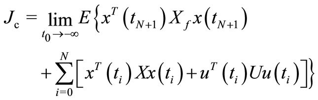 (6)
(6)
for each  and some
 ,
,  , and
, and .
.
A7  is stabilizable,
  is detectable,
  is completely observable, and
  is completely controllable.
A8 For any  the designed system holds its property to be
  -mean exponentially stable [7].
A9 A mode switching mechanism is viewed as deterministic, and yet it is unknown to the observer (like controlled by an independent actor) but allows for enough time between successive switches to leave no doubt that A1 practically holds.
Assumption A2 is made for simplicity and may be omitted if one includes a similarity transformation into the inference (thus defining new basis vectors for SOM in the state space). Assumptions A3-A5 bring the system to the realm of hybrid or multi-mode systems. One value of , denoted by
 , designates the so called adopted operating mode, which is recognized—not obligatorily albeit possibly—as a nominal operating mode, NOM. The other values
  can be viewed as specifying some alternative operating modes recognized—not obligatorily albeit possibly—as faulty operating modes, FOMs,
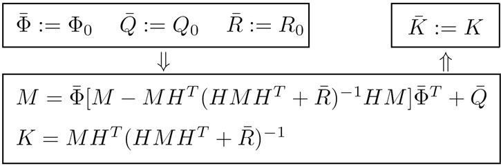
 . Assumption A7 guarantees the existence of the optimal steady-state parameters
 ,
,  ,
,  ,
,  in equations (3)-(5) for any mode. Algorithms to compute these parameters are as follows where subscript “
 ” corresponds to
 .
.
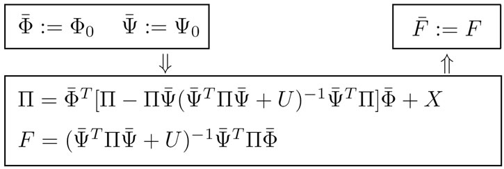
These algorithms hold when the FR function,  , is chosen to satisfy the second equality in equation (5). In this case, the assumption A8 holds if
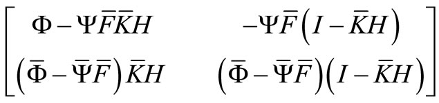
being the transition matrix for the stackable state vector  of the given system equations (1)-(5)is such that its eigenvalues lie in the open unit disc.
The problem is to identify the optimal Steady State Kalman Filter (SSKF) for any system mode that appears after a mode switch, in order to use the identification result  as a substitute for FF (
 as in Figures 4, 5 and 6 is assumed).
4. Active Principle of Adaptation
Analyzing possibilities to apply any of the adaptation principles considered above in Section 2, we put in the forefront the behavioristical aspect of the adaptive part of a system. In so doing, we notice that there are two more general principles of (or two approaches to) adaptation to be contrasted to each other:
• Passive Principle: Adaptation based on following some foremade prescriptions and so free of any tracking (and, as a sequel, without any guarantee of) the desired quality of system and its small deflection from the point of optimum, and
• Active Principle: Adaptation based on tracking (and, as a sequel, with certain guarantee of) the desired quality of system and its small deflection from the point of optimum.
Viewed from this perspective, BAM, EAM and AAM are passive, whereas PIAM and CMAM are active. Naturally, there may exist combinations of these behavioristical features in one adaptive system; however we focus on the active type of adaptation as using PIAM of Section 2 for MIMO control systems desribed in Section 3.
Original performance indices: Let  and
and  be a one-step predicted and a filtered estimate of
 , correspondingly. Evidently,
  and
and  being the errors committed by those estimators,
 (7)
(7)
 (8)
(8)
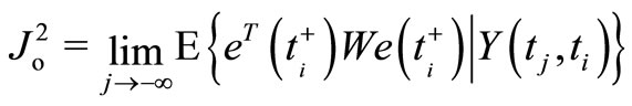
are not available in practice. They are useful in theory only when the corresponding original performanse indices (OPI) given as the limiting mean square error cost in one of two equivalent forms
 (9)
(9)
or
 (10)
(10)
whose domain includes all time-invariant one-step predicting estimators  or filtering estimators
  of
of , conditioned on the knowledge of all preceding measurements extracted from the above closed-loop system, are minimized, where
 (11)
(11)
is the standard notation for a stackable vector composed of column vectors  through
 ,
,  , and
, and  is a symmetric semi-positive definite (
 ) weighting matrix.
Problem of active principle: Given the original performance index as (9) or (10). The minimum of (9) or, equivalently, (10) is achieved for all  if and only if
  is identical to
  and
and  is identical to
  where
where  and
and  are estimates generated by the steady-state optimal (Kalman) filter
 (12)
(12)
 (13)
(13)
In (12) and (13),  ,
, 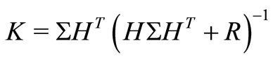 and
and  satisfies the algebraic Riccati equation
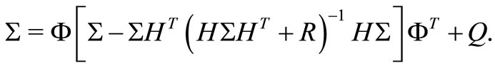 (14)
(14)
However, (9) or (10) are unfit for use in minimum seeking methods (for example, in stochastic approximation or any others used in PIAM) by virtue of (7) and (8) being unavailable. The core of our method is to form an auxiliary performance index (API), using the available values  and
and  only, so that necessary and sufficient conditions for its minimum are equivalent to those for minimum of (9) or (10).
Note that MPE methods use a performance index to be minimized, too, in the process of system (better to say, model) adaptation. However, they predict not the exact state vector  as
as  is inaccessible, but the measurement vector
 , and this is the difference between our approach and the MPE approach.
An intermediate discussion: In the equations (7) and (8), the first operand,  , can be called the hidden reference model output, while the second operand is the explicit adaptive model output to be fitted to
 . The name “hidden” comes from the fact that the “reference model output”
 , which is subject to equation (1), is unavailable.
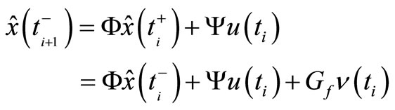
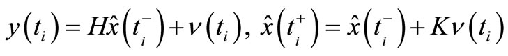
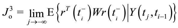
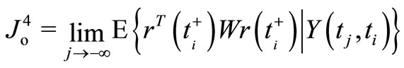
Alternative forms of OPI: If we make use of the wellknown innovation representation (12)-(13) of Data Source (1)-(2), then we can consider the following residuals
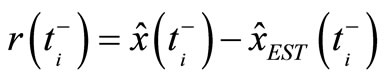 (15)
(15)
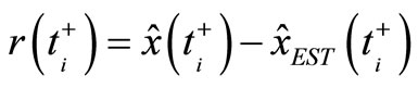 (16)
(16)
instead of errors (7)-(8). In (15)-(16), the first operand again represents the hidden reference model, in this case described by (12)-(13). Correspondingly, one can take the original performance indices in the altertative forms
 (17)
(17)
or
 (18)
(18)
equivalent to (9)-(10) in the sense that minimization of any of these performance indices leads to the optimal parameter values of the adaptive model labeled as an estimator by subscript .
.
5. Conclusions
In this paper, the author formulates a new approach called The Active Principle of Adaptation. It is intended for one class of systems, whose original performance index can be used only as a theoretical one, namely for linear time-invariant state-space stochastic MIMO filter systems, possibly included into Feedback Strategy of stochastic control or considered independently, for example, in communication systems where filtering or detecting signals is a priority.
The approach is focused on constructing an auxiliary performance index which would have two properties:
• accessibility for direct use in adaptation algorithms;
• equimodality with the original performance index.
The latter notion means that API and OPI have the same minimizing arguments. This is necessary and sufficient to guarantee (theoretically) nonbiasedness of parameter estimates. The direct way for these properties to hold is as follows:
• to form an available auxiliary process  as a substitute for any process (7), (8), (15), (16), and then
• to form the API as
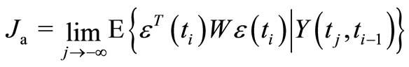
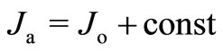
with  taken as
 ,
,  from (9), (10), (17), (18).
Such a novel set-up provides a new, broad look at this field of reasearch. Our plan for further research consists of solving the following tasks:
1) Forming the auxiliary performance index for MIMO control systems desribed in Sect. 3.
2) Studying some particular cases with different and progressively increasing levels of uncertainty, in order to determine the level, for which the API approach still remains workable.
3) Numerical experimental testing the approach and demonstrating its applicability to different applications.
4) Elucidation of the numerical properties of this approach and using the modern efficient computational techniques for its computer implementation.
6. Acknowledgements
I would like to thank Prof. B. Verkhovsky for his most helpful input, Dr. A. Murgu for his useful comments, and an anonymous reviewer for a number of corrections that improved the style of this paper.
7. References
[1] C. S. Draper, “Principles of Optimalizing Control Systems and an Application to the Inertial Combustion Engine,” ASME Publications, Mawson, 1951.
[2] R. E. Kalman, “Design of a Self-Optimizing Control Systems,” Transactions of ACME, vol. 80, 1958, pp. 468-478.
[3] A. A. Feldbaum, “The Theory of Dual Control I,” Automation and Remote Control, vol. 21, no. 9, 1961, pp. 874-883.
[4] A. A. Feldbaum, “The Theory of Dual Control II,” Automation and Remote Control, vol. 21, no. 11, 1961, pp. 1033-1039.
[5] A. A. Feldbaum, “The Theory of Dual Control III,” Automation and Remote Control, vol. 22, no. 1, 1962, pp. 1-12.
[6] A. A. Feldbaum, “The Theory of Dual Control IV,” Automation and Remote Control, vol. 22, no. 2, 1962, pp. 109-121.
[7] P. E. Caines, “Linear Stochastic Systems,” John Wiley and Sons, Inc., Hoboken, 1988.
[8] Y. Z. Tsypkin, “Adaptation and Learning in Automatic Systems,” Nauka Publications, Moscow, 1968.
[9] T. L. Lai, “Sequential Changepoint Detection in Quality Control and Dynamical Systems,” Journal of the Royal Statistical Society, Series B (Methodological), vol. 57, no. 4, 1995, pp. 613-658.
[10] P. Ansay, M. Gevers and V. Wertz, “Closed-Loop or Open-Loop Models in Identification for Control?” In: P. Frank, Ed., CD-ROM Proceedings of 5th European Control Conference, Karlsruhe, 31 August-3 September 1999, File F0544.
[11] O. Grospeaud, T. Poinot and J. C. Trigeassou, “Unbiased Identification in Closed-Loop by an Output Error Technique,” In: P. Frank, Ed., CD-ROM Proceedings of 5th European Control Conference, Karlsruhe, 31 August-3 September 1999, File F0792.
[12] L. Ljung, “Convergence Analysis of Parametric Identification Methods,” IEEE Transactions on Automatic Control, vol. AC-23, no. 5, 1978, pp. 770-783. doi:10.1109/ TAC.1978.1101840
[13] A. H. Jazwinski, “Stochastic Processes and Filtering Theory,” Academic Press, Cambridge, 1970.
[14] H. Kaufman and D. Beaulier, “Adaptive Parameter Identification,” IEEE Transactions on Automatic Control, vol. AC-17, no. 5, 1972, pp. 729-731. doi:10.1109/TAC.1972. 1100111
[15] H. Cramér and M. R. Leadbetter, “Stationary and Related Stochastic Processes. Sample Function Properties and Their Applications,” John Wiley and Sons, Inc., Hoboken, 1967.