ABSTRACT

The Data Timed Sending (DTS) protocol contributes to the energy savings in Wireless Sensor Networks (WSNs) and prolongs the sensor nodes’ battery lifetime. DTS saves energy by transmitting short packets, without data payload, from the sensor nodes to the base station or the cluster head according to the Time Division Multiple Access (TDMA) scheduling. Placing the short packets into appropriate slots and subslots in the TDMA frames transfers the information about the measured values and node identity. This paper presents the proof of concept of the proposed DTS protocol and provides verification of the energy savings using the QualNet^® communication simulation platform (QualNet) and the Sun^TM Small Programmable Object Technology (Sun SPOT) testbed platform (for single hop and multi hop scenarios). The simulations and the testbed measurements confirm that the DTS protocol can provide energy savings up to 30% when compared with the IEEE 802.15.4 standard in unslotted Carrier Sense Multiple Access with Collision Avoidance (CSMA-CA) mode at 2.4 GHz frequency band.

1. Introduction

The Wireless Sensor Networks (WSNs) have become an important tool for gathering information in all areas of the human life. A WSN is a network made of small size and low-power sensor nodes with capabilities to collect, process, and wirelessly transmit various types of data. The WSN platforms introduce different routings [1-3], power management [4-9], and synchronization protocols [10-15]. The specific WSN requirements contribute to the development and implementation of various operating systems [16] and applications [17]. The possible applications cover a wide range of areas, such as environmental monitoring, medical care, smart homes, robot controlling, security, public safety, surveillance, commercial applications, tracking, identification, personalization, etc.

A typical WSN consists of spatially distributed autonomous battery powered sensor nodes, which sense and cooperatively pass their data to a base station directly (single hop) or through the intermediate nodes (multi hop). Changing or recharging the batteries on remote nodes is a difficult, time-consuming and expensive task. It is very important for the WSNs to reduce the amount of energy consumption in each node, which in turn extends the network lifetime and reduces the number of the necessary interventions. Some energy saving solutions reduce the packet loss ratio and the length of a packet’s route by exploiting energy aware routing [6,7,9,18,19], whereas others are oriented towards energy harvesting methods [20-22]. The energy aware routing improves the energy conservation in conditions of congestion or link failure.

The Data-Timed Sending (DTS) protocol improves the energy efficiency in WSNs by usage of short packets without data payload. DTS uses Time Division Multiple Access (TDMA) to transfer the measured values. Reference [23] presents the preliminary evaluation of the DTS protocol. The evaluation in [23] was carried out only on the basis of C++ simulation about single hop scenario. This paper presents both simulation and practical testbed results about the energy savings of the DTS protocol in multi hop topology when compared to the unslotted Carrier Sense Multiple Access with Collision Avoidance (CSMA-CA) protocol according to the IEEE 802.15.4- 2006 standard. The simulations are performed on a Qual Net simulator, and the testbed implementation is realized on a Sun^TM Small Programmable Object Technology (Sun SPOT) WSN testbed platform. This paper is organized as follows. The second section describes the DTS protocol. The third section gives the power consumption analysis. The fourth section presents the simulation scenarios and results. The fifth section describes the Sun SPOT testbed platform, whereas the sixth section provides the results of the energy consumption comparison. The seventh section gives the conclusions.

2. DTS Protocol

The DTS is TDMA based protocol. It can support single hop and multi hop topologies. When a DTS-enabled WSN uses single hop topology, it is organized as a star network where every remote sensor node sends packets directly to the base station. When a DTS-enabled WSN uses multi hop topology, it is organized as a cluster network where nodes are grouped in clusters. Each cluster has one cluster-head node. In the cluster network every remote sensor node sends packets to its cluster-head, which acts as an intermediate node to the base station.

2.1. DTS in Single Hop Topology

In a single hop scenario the time is organized in frames, where each frame is divided in N slots, and each slot is divided in P + 1 subslots, as shown in Figure 1. The parameter N is the number of the remote sensor nodes associated with the base station and P is the number of the possible values of the measured phenomenon. Each node has dedicated slot and each measured value has dedicated subslot. During each frame, each node sends one short packet (without data payload) about the measured value during the previous frame. The node transmits short packet in the slot and the subslot that correspond to the node’s ordinal number and the measured value, respectively. The base station can recognize which node has sent the short packet and what is the measured value only by its positioning within the frame. The requirements of

a particular WSN application determine the length of the frames and the number of the slots and subslots. The DTS protocol synchronizes the nodes with the base station [24]. The synchronization mechanism works by broadcasting the resynchronization packets from the base station in regular resynchronization intervals. The duration of the resynchronization interval depends on the application requirements.

The duration of the short packet as well as the duration of the resynchronization packet must be less than the duration of one subslot. The minimum packet’s size depends on the hardware characteristics of the node’s radio (8 bytes for the Sun SPOT’s radio chip). The size of the short and the resynchronization packets is usually equal to the minimum packet’s size allowed by the node’s radio chip in order to maximize the energy savings (shorter packet keeps the radio less time switched on).

The sensor nodes are in sleeping mode most of the time and they wake up only to send the short packet to the base station, to take new measurement or to receive a resynchronization packet. The base station broadcasts the resynchronization packet in a subslot determined by the resynchronization interval. Therefore, the number of the subslots is P + 1.

The statistical synchronization protocols [10,11,14], can achieve a synchronization error of less than 10 microseconds. With such small errors, a 30 second long slot can contain 60,000 subslots where each subslot is wide enough to accept a 15 byte packet at 250 kb/s bit rate along with two error margins. It allows using the single subslot not just for one value of one measured phenomenon, but for a combination of values of several phenomena (e.g. temperature, air pressure, and humidity). In cases of environmental monitoring, the sensor should collect data with rate at least equal to changes of environmental conditions noticeable for humans or other living organisms (usually once in 5 to 10 minutes) [25]. Due to limited number of packet transmissions and synchronization constraints [24], the DTS protocol is suitable for WSN applications that do not demand extremely high bit rates.

2.2. DTS in Multi Hop Topology

In a multi hop scenario the time is organized in frames, where each frame is divided in two subframes, i.e., in subframe A and subframe B, as shown in Figure 2. The subframe A covers the time when the remote sensor nodes send packets to their corresponding cluster-head node, and the subframe B covers the time when the cluster-head nodes send packets to the base station.

The subframe A is divided in R slots, and each slot is divided in M + 1 subslots, as shown on Figure 3. The parameter R is the number of the remote sensor nodes

associated with one cluster-head node, and M is the number of the possible values of the measured phenomenon. Each remote sensor node has dedicated slot and each measured value has dedicated subslot. During each subframe A, each remote sensor node sends one short packet (without data payload) with information about the measured value during the previous frame. The remote sensor node transmits short packet in the slot and the subslot that correspond to the remote sensor node’s ordinal number and the measured value, respectively. The cluster-head node can recognize which node has sent the short packet and what the measured value is only by its positioning within the subframe A. All clusters are far apart from each other or they use different frequency channels, so the subframe A is common for all clusterheads.

The subframe B is divided in C slots, each slot is divided in R subslots, and each subslot is divided in M+1 sub-subslots, as shown in Figure 4. The required diapason and granulation of the measured phenomenon determines the number of the sub-subslots. The parameter C is the number of the cluster-head nodes associated with the base station, R is the number of the remote sensor nodes associated with one cluster-head node, and M is the number of the possible values of the measured phenomenon. Each cluster-head node has dedicated slot, each remote sensor node has dedicated subslot, and each measured value has dedicated sub-subslot. During each subframe B, each cluster-head node sends R short packets (without data payload) about the measured value during the previous frame. The cluster-head node transmits short packet in the slot, subslot, and the sub-subslot that correspond to the cluster-head node’s ordinal number, remote sensor node’s ordinal number, and the measured

value, respectively. The base station can recognize which cluster-head node has sent the short packet, which remote sensor node represents that short packet, and what the measured value is only by packet’s position within the subframe B.

The synchronization mechanism works by broadcasting the resynchronization packets from the base station in regular resynchronization intervals.

The remote sensor nodes are in sleeping mode most of the time and they wake up only to send the short packet to the cluster-head node, to take new measurement or to receive a resynchronization packet. The base station broadcasts the resynchronization packet in a subslot or subsubslot determined by the resynchronization interval. Therefore, the number of the subslots and sub-subslots is M + 1.

The DTS protocol is convenient for static rather than ad hoc network scenarios since the software reflects the topology and need to be upgrade if the topology changes.

3. Power Consumption

The characteristics of the sensor nodes have a significant impact on its power consumption. The usual design approach for ultra low-powered devices, such as sensor nodes, is to minimize the average current draw by spending as much time as possible in a low-power consumption mode so-called sleep mode. In the active period, the device intensively draws current from its battery. After the active period, the device returns into a sleeping mode.

3.1. Distribution of Power Consumption

The sensor node comprises four entities that are major power consumers, i.e., the radio, the microcontroller, the interface circuitry and the software running on the microcontroller. They are briefly described in the following text.

• Radio—the WSN nodes are devices with limited resources. They tend to use simple transceivers (TRX) that cannot receive and transmit simultaneously. The transmitting current draws are at a scale of tens of milliamps, whereas the low-power mode current draw is at a scale of microamps [4]. Since the radio usage consumes the majority of the node energy [26], the development of low energy consumption Medium Access Control (MAC) protocols is of great importance for WSNs.

• Microcontrollers—microcontrollers comprise a Central Processor Unit (CPU), timers, Universal Asynchronous Receivers Transmitters (UARTs), inputs, outputs, etc. Power consumption of a CPU depends on its implementation, i.e., on the application demands. The current draw in active mode exceeds hundred milliamps, whereas in a low-power mode it is at a scale of microamps.

• Interface Circuitry—this circuit depends on the application. It includes light indicators, external analog or digital inputs and outputs, relays, etc. The current draw varies in a range from tens to hundred of milliamps [4]. The microcontroller needs to be awake to change the state of an output, but it can turn to sleep leaving an output device powered on.

• Software—the software can manage the switching on and off of the processes. The software can be designed by the user as an application or by the manufacturer as an operating system. The overall software is designed to minimize the power consumption.

3.2. Power Consumption of IEEE 802.15.4 with 2.4 GHz Unslotted CSMA-CA

The IEEE 802.15.4 standard defines a symbol as the smallest operational time unit. Table 1 lists the parameters of the IEEE 802.15.4 unslotted CSMA-CA in the 2.4 GHz band [27].

When a node needs to transmit a data packet, it waits for a random time and then performs Clear Channel Assessment (CCA), i.e., hears if the channel is idle or busy. If the channel is idle, the node transmits the data packet. If the channel is busy, the node backs off, i.e., waits for another random time before it performs the next CCA. The node repeats this procedure, but if the algorithm ex-

ceeds the maximum allowed number of backoffs, then the transmission is canceled [27]. The average number of backoffs N_AvBack is derived from the analysis based on [28].

Probability that a node transmits in a CCA period, A_TrCCA is given with:

(1)

where T_AvChOccup is average channel occupation time in a fixed time period, T_{FixTimePeriod}. The designer defines both T_AvChOccup and T_{FixTimePeriod}.

Probability A_CC that a channel is idle after the first backoff interval, for network with N_S sensor nodes, is given with:

. (2)

According to the IEEE 802.15.4, the overall backoff time can be comprised of up to five backoff intervals plus associated CCA periods. In the case of maximum five backoff intervals [27], the probability of transmission, A_TR is:

. (3)

Then, the average number of backoffs, N_AvBack becomes:

. (4)

The unslotted CSMA-CA average receiver power consumption, P_UnAvRX is:

(5)

where P_RX is active receiver power consumption, T_StRX is the receiver start-up time, T_CCA is time for performing CCA, T_ACK is acknowledgment packet duration (if acknowledgment is required), and T_SndUn is a interval in which node sends one data packet.

The unslotted CSMA-CA average transmitter power consumption, P_UnAvTX is defined as:

(6)

where P_TX is active transmitter power consumption, T_StTX is the transmitter start-up time and T_DAT is the duration of the data packet.

3.3. Power Consumption of DTS

The DTS protocol does not perform a CCA listening and it uses short packets instead of long IEEE 802.15.4 data packets. DTS requires synchronization among the nodes and the base station. Base station broadcast resynchronization packets in order to achieve the synchronization. The clock of the base station is designated as a reference clock. The base station broadcasts the resynchronization packet every time its resynchronization timer reaches the value of the resynchronization interval, T_RI. Then, the base station sets its resynchronization timer back to the zero value and starts a new counting. All nodes simultaneously receive the resynchronization packets and synchronize their timers with the base station timer. To overcome the uncertainty between the node’s local notion of time and that of the base station, the node turns on its receiver shortly (i.e. T_Guard) before its timer reaches the T_RI value. Longer values of the resynchronization interval T_RI result in greater drift accumulation from the clock frequency errors.

The DTS average receiver power consumption, P_DTSAvRX is only a consequence of the reception of the resynchronization packet and is defined as:

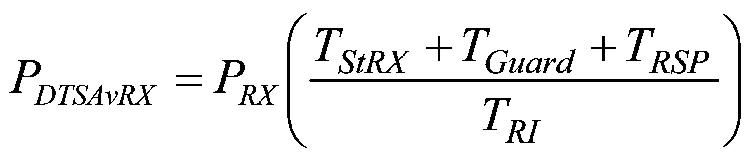(7)

where P_RX and T_StRX are active receiver power consumption and  receiver start-up time respectively, and T_RSP is the duration of the resynchronization packet.

The DTS average transmitter power consumption, P_DTSAvTX is defined as:

(8)

where P_TX is active transmitter power consumption, T_StTX is the transmitter start-up time, T_DTS is the duration of short DTS packet and T_SndDTS is frame duration in which the node sends one short DTS packet.

3.4. Energy Consumption Challenges

The rapid and sudden changes of the current draw at the WSN nodes impose serious difficulties in their energy consumption monitoring. The consumed energy E_n in time interval T that starts at t = t₀ and ends at t = t₀ + T is given with:

(9)

where u_b(t) is the voltage of the battery and i_b(t) is the battery current draw. Battery voltage does not change drastically although the current can vary from microamps to tens or hundreds of milliamps (more than three orders of magnitude) in the scale of microseconds [29]. Rapid change of the current draw is mostly a consequence of the occasionally awakening of the node to take a reading or send a packet and sleeping on the remainder of the time. The current variation causes variation of the consumed energy in the scale of microseconds. Simple approximations of nodal energy consumption derived from estimates of duty cycle and receiving/transmitting rates (5)-(8) do not capture entirely the low-level system power profile of the WSNs [29]. A node can exhibit a bewildering array of power profiles depending on its application profile. Another problem is short-duration power spikes during periods of brief activities of the operating system or background processes. Additional inconsistency of the current draw is due to the temperature variation, which affects the current leakage [29]. These are the motivations to implement a given WSN protocol on a real platform in order to discover its true performances.

4. Simulation Scenario

The proof of concept for the energy efficiency of the proposed DTS protocol was confirmed with simulation setup performed with QualNet. QualNet can model scenarios for large number of nodes by taking advantage of the latest hardware and parallel computing techniques. It includes advanced models for the wireless environment to enable more accurate modeling of real-world wireless networks. This section presents the simulation result used for comparison of energy consumption of DTS with IEEE 802.15.4 unslotted CSMA-CA protocols.

4.1. Simulation Architecture and Scenario

Simulation scenarios include cases for different number of remote sensor nodes grouped in clusters, as shown in Figure 5. Remote sensor nodes from one cluster send packets to their cluster-head node, which in turn sends packets to the base station. Tables 2 and 3 list the parameters of the IEEE 802.15.4 and DTS.

The number of the clusters is 5. In this scenario, the clusters are sufficiently distant from each other to ex-

clude interference. (In reality, another way to exclude interference is to allocate different frequency channels to clusters.) Connection between each remote sensor node and the base station is multi hop. Simulations are repeated 10 times, starting with a total of 10 remote sensor nodes (2 remote nodes per one cluster-head), and ending with a total of 100 remote sensor nodes (20 remote nodes per one cluster-head). Each remote sensor node takes measurement readings and sends a packet once in 20 minutes (which corresponds to the realistic environmental monitoring scenarios, e.g. air temperature).

The simulation setup was used to confirm the advantages of the DTS compared with the IEEE 802.15.4. QualNet simulator runs scenario with IEEE 802.15.4 unslotted CSMA-CA protocol on PHY and MAC layers and utilizes ZigBee (variation of Ad hoc On-Demand Distance Vector (AODV)) as routing protocol. In DTS case, the QualNet simulator runs scenario with DTS protocol on PHY, MAC, and routing layers.

4.2. Simulation Results

The average energy consumption per remote sensor node shows the energy efficiency of both protocols. Figures 6 and 7 give the average energy consumption per remote

sensor node and the standard deviation of the average energy consumption per node, respectively, for 10, 20, … to 100 total number of remote sensor nodes. Table 4 summarizes the simulation results.

Simulations show that DTS protocol consumes approximately 30% less energy than IEEE 802.15.4 unslotted CSMA-CA protocol, and energy savings do not depend on the total number of remote sensor nodes. Simulations also show that DTS protocol has constant and lower standard deviation of the energy consumption than IEEE 802.15.4 unslotted CSMA-CA, whose standard deviation of the energy consumption increases with larger number of remote sensor nodes.

For IEEE 802.15.4 scenario, the standard deviation of the energy consumption per remote node experiences approximately linear growth as total number of remote sensor nodes increase. This is due to increase in packet collisions and medium occupancy as total number of remote sensor nodes increase. In such conditions some remote nodes do not receive acknowledgement packet and perform retransmission (spend more energy than average), whereas other remote nodes detect busy channel consequently several times and disclaim transmission (spend less energy than average). For DTS scenario, each transmission has dedicated time slot, so remote nodes neither retransmit packets nor disclaim transmission of the packets.

5. Testbed Platform

Sun SPOT testbed was designed to compares the energy

consumption between the DTS and IEEE 802.15.4 unslotted CSMA-CA and to prove the energy efficiency of the DTS in realistic environment. The testbed works in a laboratory indoor environment. The testbed WSN application measures the air temperature and luminosity. This section presents the testbed scenarios and results.

5.1. Testbed Architecture and Scenario

The testbed consists of 8 Sun SPOTs that act as remote sensor nodes, 2 Sun SPOTs that act as cluster-head nodes, and one base station attached to the laptop host computer via Universal Serial Bus (USB) cable, as shown in Figure 8. The base station serves as a gateway to the host computer. The cluster-head Sun SPOTs are labeled as cluster-head nodes 1 and 2. Remote Sun SPOTs are labeled as remote nodes 1, 2, … to 8. The remote nodes were placed at distances less than 10 m from their corresponding cluster-heads, and the cluster-heads were placed at distances less than 10 m from the base station. The Sun SPOTs are Sun Microsystems-2008 model. Table 5 lists Sun SPOTs’ hardware characteristics [30- 33]. Remote nodes 1 to 4 are connected to the cluster-head node 1, and remote nodes 5 to 8 are connected to the cluster-head node 2.

Communication between remote nodes 1 to 4 and the cluster-head 1 is set up on IEEE 802.15.4 radio channel 11, and communication between remote nodes 5 to 8 and the cluster-head 2 is set up on IEEE 802.15.4 radio channel 12. Communication between cluster head nodes 1, 2, and the base station is on IEEE 802.15.4 radio channel 25. When testbed works with DTS protocol, the base station sends resynchronization packets at IEEE 802.15.4 radio channel 25.

During the IEEE 802.15.4 measurement, the remote sensor nodes use an energy saving sleep mode and wake up once in every 1200 s to take temperature and luminosity measurement and to send data packet to the base station via their corresponding cluster-head nodes. The PHY and MAC layers works with IEEE 802.15.4 unslotted CSMA-CA standard, and the routing protocol is 6LoWPAN (IPv6 compatible Low power Wireless Personal Area Networks). In terms of energy efficiency, 6LoWPAN and ZigBee are very similar, i.e., the both are designed for small low-power devices with limited processing capabilities. After measuring and sending the

packet, the sensor node is going back to sleep mode.

During the DTS measurements, the remote sensor nodes use an energy saving sleep mode and wake up once in every 20 minutes to take temperature and luminosity measurement and to send short DTS packet to their corresponding cluster-head nodes. After the cluster-heads receive short DTS packets from all remote nodes in their cluster, they begin to send short DTS packets to the base station. All remote and cluster-head nodes also wake up once in every 60 minutes to receive the short resynchronization DTS packet. In this mode, DTS protocol covers the PHY layer, MAC layer, and the routing procedure.

Tables 6 and 7 list the parameters of the IEEE 802. 15.4 and DTS scenarios. Table 8 lists DTS TDMA scheduling of the remote and cluster-head nodes. The terms in Table 8 are consistent with the terms described in Figures 2-4.

During the testbed measurements, each remote Sun SPOT records the battery voltage level on its flash memory every 5 minutes. The measurement run until the battery is completely discharged. Based on the records in flash memory about their battery voltages, the battery discharge curves are plotted for each remote Sun SPOT in each regime of its operation (IEEE 802.15.4 or DTS),

providing an evaluation of the energy consumption. The most significant point of the curve is the moment when the voltage drops to a critical value at which the remote Sun SPOT stops to work.

Sun SPOTS are manufactured with embedded IEEE 802.15.4 unslotted CSMA-CA (PHY and MAC layers) and with embedded 6LoWPAN routing protocol. But, for the DTS evaluation, the existing network software is replaced with custom made software in order to implement the DTS functionalities.

5.2. Testbed Results

The discharge curves for each remote Sun SPOT provides evaluation of its energy consumption. Figures 9(a) and (b) show the discharge curve of the remote Sun SPOT 1 when it works with the IEEE 802.15.4 unslotted CSMA-CA and DTS protocol, respectively. The critical points C_Unslotted1 and C_DTS1 mark the time and the battery voltage level of the remote Sun SPOT 1, when it stops to work with the IEEE 802.15.4 unslotted CSMA-CA and DTS protocol, respectively. The flat lines give the last recorded voltage levels in remote Sun SPOT 1 flash memory before its battery is fully discharged. The time difference between the critical points C_DTS1 and C_Unslotted1, TD₁, gives the quantity of the energy savings. For the remote Sun SPOT 1, the time difference is 27%, which indicates that the DTS achieves 27% energy savings when compared with the 2.4 GHz, unslotted CSMA-CA IEEE 802.15.4. The remote Sun SPOTs 2 to 8 have similar discharge curves and Figure 10 shows their energy savings. Table 9" target="_self"> Table 9 summarizes the results from the testbed platform.

The difference among the discharging times of remote Sun SPOTs 1 to 8, when they are working with the IEEE 802.15.4 or DTS, is due to the different individual battery characteristic, hardware imperfection and other external influences. However, it is evident that DTS pro-

vides energy savings approximately around 30%.

6. Conclusion

This paper presents proof of concept for DTS energy efficient protocol and gives a QualNet simulation and Sun SPOT testbed verification for significant energy savings of 30% achieved when compared with IEEE 802.15.4 unslotted CSMA-CA. DTS protocol uses TDMA approach for communication combined with short packets without data payload. The simulation and the testbed results are consistent and proof the energy efficiency of the DTS in WSNs.

7. Acknowledgements

This work was supported in part by the European Commission FP7 ProSense project under Grant agreement no. 205494.

REFERENCES

- S. K. Singh, M. P. Singh and D. K. Singh, “Routing Protocols in Wireless Sensor Networks—A Survey,” International Journal of Computer Science & Engineering Survey, Vol. 1, No. 2, 2010, pp. 63-83. doi:10.5121/ijcses.2010.1206
- L. J. G. Villalba, A. L. S. Orozco, A. T. Cabrera and C. J. B. Abbas, “Routing Protocol in Wireless Sensor Networks,” Sensors, Vol. 9, No. 11, 2009, pp. 8399-8421. doi:10.3390/s91108399
- Y. Al-Obaisat and R. Braun, “On Wireless Sensor Networks: Architectures, Protocols, Applications, and Management,” Proceedings of the AusWireless 2006 Conference, Sydney, 13-16 March 2006, pp. 1-11.
- A. Norouzi and A. Sertbas, “An Integrated Survey in Efficient Energy Management for WSN using Architecture Approach,” International Journal of Advanced Networking and Applications, Vol. 3, No. 1, 2011, pp. 968- 977.
- M. D. Francesco, G. Anastasi, M. Conti, S. K. Das and V. Neri, “Reliability and Energy-Efficiency in IEEE 802.15. 4/Zigbee Sensor Networks: An Adaptive and Cross-Layer Approach,” Selected Areas in Communications, Vol. 29, No. 8, 2011, pp. 1508-1524. doi:10.1109/JSAC.2011.110902
- S. K. Singh, M. P. Singh and D. K. Singh, “Energy-Efficient Homogeneous Clustering Algorithm for Wireless Sensor Network,” International Journal of Wireless & Mobile Networks, Vol. 2, No. 3, 2010, pp. 49-61. doi:10.5121/ijwmn.2010.2304
- M. Liu, J. Cao, G. Chen and X. Wang, “An EnergyAware Routing Protocol in Wireless Sensor Networks,” Sensors, Vol. 9, No. 1, 2009, pp. 445-462. doi:10.3390/s90100445
- H. Abusaimeh and S. H. Yang, “Dynamic Cluster Head for Lifetime Efficiency in WSN,” International journal of Automation and Computing, Vol. 6, No. 1, 2009, pp. 48- 54. doi:10.1007/s11633-009-0048-0
- A. G. A. Elrahim, H. A. Elsayed, S. E. Ramly and M. M. Ibrahim, “An Energy Aware WSN Geographic Routing Protocol,” Universal Journal of Computer Science and Engineering Technology, Vol. 1, No. 2, 2010, pp. 105-111.
- C. Lenzen, T. Locher and R. Wattenhofer, “Tight Bounds for Clock Synchronization,” Journal of the ACM (JACM), Vol. 57, No. 2, 2010, Article No. 8. doi:10.1145/1667053.1667057
- C. Lenzen, P. Sommer and R. Wattenhofer, “Optimal Clock Synchronization in Networks,” Proceedings of the 7th ACM Conference on Embedded Networked Sensor Systems, Berkeley, 4-6 November 2009, pp. 225-238. doi:10.1145/1644038.1644061
- P. Sommer and R. Wattenhofer, “Gradient Clock Synchronization in Wireless Sensor Networks,” Proceedings of the 8th ACM/IEEE International Conference on Information Processing in Sensor Network 2009, San Francisco, 13-16 April 2009, pp. 37-48.
- S. Ganeriwal, R. Kumar and M. B. Srivastava, “Timing-Sync Protocol for Sensor Networks,” Proceedings of the 1st International Conference on Embedded Networked Sensor Systems, Los Angeles, 5-7 November 2003, pp. 138-149. doi:10.1145/958491.958508
- M. Maroti, B. K. G. Simon and A. Ledeczi, “The Flooding Time Synchronization Protocol,” Proceedings of the 2nd International Conference on Embedded Networked Sensor Systems, Baltimore, 3-5 November 2004, pp. 39- 49. doi:10.1145/1031495.1031501
- S. Ganeriwal, D. Ganesan, H. Sim, V. Tsiatsis and M. B. Srivastava, “Estimating Clock Uncertainty for Efficient Duty-Cycling in Sensor Networks,” IEEE/ACM Transactions on Networking, Vol. 17, No. 3, 2009, pp. 842-856. doi:10.1109/TNET.2008.2001953
- M. O. Farooq and T. Kunz, “Operating Systems for Wireless Sensor Networks: A Survey,” Sensors, Vol. 11, No. 6, 2011, pp. 5900-5930. doi:10.3390/s110605900
- C. F. Garcia-Hernandez, P. H. Ibarguengoytia, J. Garcia-Hernandez and J. A. Perez-Diaz, “Wireless Sensor Networks: A Survey,” International Journal of Advanced Networking and Applications (IJANA), Vol. 7, No. 3, 2007, pp. 264-273.
- K. Padmanabhan and P. Kamalakkannan, “A Study on Energy Efficient Routing Protocols in Wireless Sensor Networks,” European Journal of Scientific Research, Vol. 60, No. 4, 2011, pp. 517-529.
- S. Ito and K. Yoshigoe, “Performance Evaluation of Consumed Energy-Type-Aware Routing (CETAR) for Wireless Sensor Networks,” International Journal of Wireless & Mobile Networks, Vol. 1, No. 2, 2009, pp. 93- 104.
- R. Nallusamy and K. Duraiswamy, “Solar Powered Wireless Sensor Networks for Environmental Applications with Energy Efficient Routing Concepts—A Review,” Information Technology Journal, Vol. 10, No. 1, 2011, pp. 1-10.
- Z. G. Wan, Y. K. Tan and C. Yuen, “Review on Energy Harvesting and Energy Management for Sustainable Wireless Sensor Networks,” Proceedings of the 13th IEEE International Conference on Communication Technology, Jinan, 25-28 September 2011, pp. 362-367. doi:10.1109/ICCT.2011.6157897
- W. Seah, Z. Eu and H. Tan, “Wireless Sensor Networks Powered by Ambient Energy Harvesting (WSN-HEAP)- Survey and Challenges,” Proceedings of the 1st International Conference on Wireless Communication, Vehicular Technology, Information Theory and Aerospace & Electronic Systems Technology, Aalborg, 17-20 May 2009, pp. 1-5. doi:10.1109/WIRELESSVITAE.2009.5172411
- K. Chomu and L. Gavrilovka, “Data-Timed Sending Method—Solution for Higher Energy Efficiency,” Proceedings of the 25th National Symposium of Telecommunications and Computer Networks, Warsaw, 16-18 September 2009, pp. 1488-1497.
- K. Chomu and L. Gavrilovka, “Synchronization Impact on the Performance of Data-Timed Sending (DTS) Based Wireless Sensor Networks,” Proceedings of the 11th IEEE International Symposium on A World of Wireless, Mobile and Multimedia Networks, Montreal, 14-17 June 2010, pp. 682-687. doi:10.1109/WOWMOM.2010.5534954
- J. Polastre, R. Szewcyk, A. Mainwaring, D. Culler and J. Anderson, “Analysis of Wireless Sensor Networks for Habitat Monitoring,” In: C. S. Raghavendra, K. M. Sivalingam and T. Znati, Eds., Wireless Sensor Networks, Kluwer Academic Publishers, Boston, 2004, pp. 399-423.
- B. Bates, A. Keating and R. Kinicki, “Energy Analysis of Four Wireless Sensor Network MAC Protocols,” Proceedings of the 6th International Symposium on Wireless and Pervasive Computing, Hong Kong, 23-25 February 2011, pp. 1-6. doi:10.1109/ISWPC.2011.5751321
- IEEE 802.15.4-2006 Standard, IEEE Society, 2006.
- N. F. Timmons and W. G. Scanlon, “Analysis of the Performance of IEEE 802.15.4 for Medical Sensor Body Area Networking,” Proceedings of the 1st IEEE International Conference on Sensor and Ad Hoc Communications and Networks (SECON’04), Santa Clara, 4-7 October 2004, pp. 16-24. doi:10.1109/SAHCN.2004.1381898
- X. Jiang, P. Dutta, D. Culler and I. Stoica, “Micro Power Meter for Energy Monitoring of Wireless Sensor Networks at Scale,” Proceedings of the 6th Information Processing in Sensor Networks, Cambridge, 25-27 April 2007, pp.186-195. doi:10.1145/1236360.1236386
- Sun Microsystems, Inc., SunTM SPOT Theory of Operation, 2009. http://sunspotworld.com/docs/Red/SunSPOT-TheoryOfOperation.pdf
- Sun Microsystems, Inc., SunTM SPOT Owner’s Manual, 2009. http://www.sunspotworld.com/docs/Red/SunSPOT-OwnersManual.pdf
- Sun Microsystems, Inc., SunTM SPOT Small Programmable Object Technology (Sun SPOT) Developer’s Guide, 2009. http://www.sunspotworld.com/docs/Red/spot-developers-guide.pdf
- 2.4 GHz IEEE 802.15.4/ZigBee-ready RF Transceiver CC2420, Chipcon Products from Texas Instruments, Inc. 2010. http://www.ti.com/lit/ds/symlink/cc2420.pdf