Wireless Sensor Network
Vol. 4 No. 10 (2012) , Article ID: 23700 , 7 pages DOI:10.4236/wsn.2012.410035
Low Power Transceiver Design Parameters for Wireless Sensor Networks
College of Information and Electrical Engineering, China Agricultural University, Beijing, China
Email: johnodey@yahoo.com
Received August 22, 2012; revised September 24, 2012; accepted September 30, 2012
Keywords: Transceiver Design Parameters; Low Power Wireless Sensor Networks; Energy Model
ABSTRACT
Designing low power sensor networks has been the general goal of design engineers, scientist and end users. It is desired to have a wireless sensor network (WSN) that will run on little power (if possible, none at all) thereby saving cost, and the inconveniences of having to replace batteries in some difficult to access areas of usage. Previous researches on WSN energy models have focused less on the aggregate transceiver energy consumption models as compared to studies on other components of the node, hence a large portion of energy in a WSN still get depleted through data transmission. By studying the energy consumption map of the transceiver of a WSN node in different states and within state transitions, we propose in this paper the energy consumption model of the transceiver unit of a typical sensor node and the transceiver design parameters that significantly influences this energy consumption. The contribution of this paper is an innovative energy consumption model based on simple finite automata which reveals the relationship between the aggregate energy consumption and important power parameters that characterize the energy consumption map of the transceiver in a WSN; an ideal tool to design low power WSN.
1. Introduction
The emerging field of wireless sensor networks (WSN) creates a new and interesting paradigm in the way we interact with our environment. Typically, a WSN node performs several functions, including; sensing environmental physical parameters, processing the raw data locally to extract characteristic features of interest, storing this information momentarily, and using a wireless link to transmit the information to its neighbors [1,2]. Each node in the sensor network node consists of four components (Figure 1); a sensor which connects the network to physical world, computation part which consists of microcontroller or microprocessor in some application responsible for control of the sensors, a transceiver for communicating between nodes and base station, and power supply which is usually from batteries. Energy consumption is a requirement for all the components of the WSN node to work, and since a wireless sensor node is typically battery operated, it is therefore energy constrained. Even with the most energy dense state of the arts battery, the operational life of a miniaturized system, capable of sensing, storage and wireless telemetry, is relatively short, requiring periodic maintenance by personnel which is costly and in many cases prohibitive and/or dangerous [1].
Much work has been done on low-powered sensor nodes and their communication abilities. Some examples are schemes handling, the reduction of communication, effective routing and multihop schemes, the reactive partial waking up of WSN nodes [1-13]. Most researches are focused on performance comparisons and trade-off studies between various low-energy routing and self-organization protocols, [3] while keeping other system parameters fixed.
One of the most important questions regarding WSN is what the power consumption at the sensor node must be and how much this affect the life expectancy of such a network [4]. In order to design a low power WSN, it is important to understand the power dissipation characteristics of the sensor node and the energy consumption metrics of the network as a whole.
The transceiver consumes bulk of the power available to a sensor node [1]. However previous energy consumption researches have focused on a generalized energy model without a clear indication of how the transceiver components affect the overall energy consumption of the sensor node. As a result, very little has been revealed about the relationship between the transceiver power characteristics and aggregate energy consumption.
A WSN transceiver is made up of the front end, back end and assisting electronic components (see Figure 2)
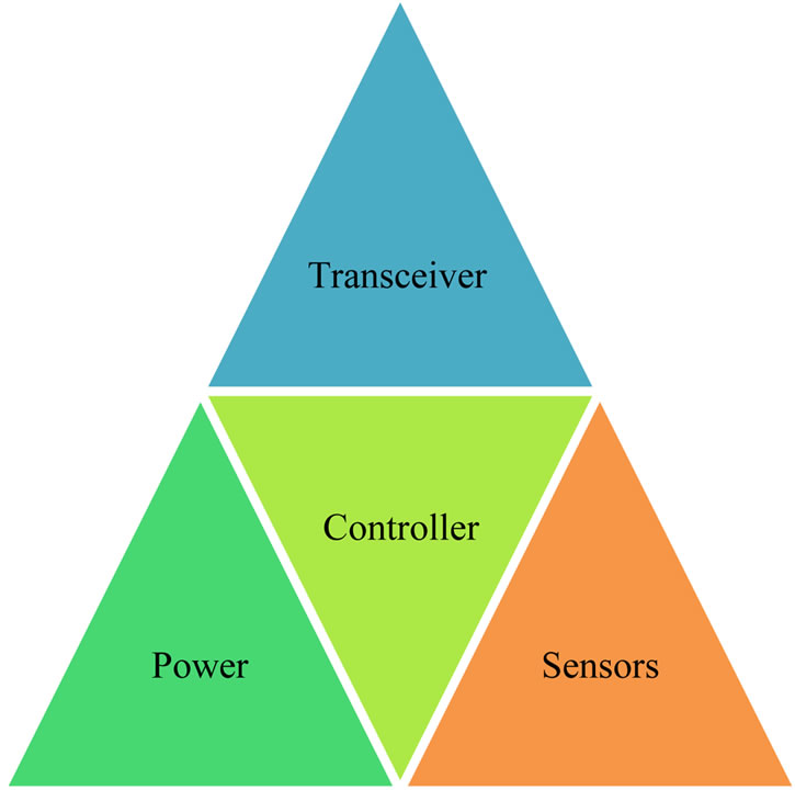
Figure 1. Components of a wireless sensor node.
like Digital/Analog Converters (DACs) and Analog/ Digital Converters (ADCs), Mixers, frequency synthesizers, voltage control oscillators (VCO), phase locked loops (PLL) and power amplifiers, and all these need power to work. There are wide ranges of choices of parameters and trade-offs necessary when designing WSN node and making the optimal choices of components and design considerations goes a long way to affect the energy consumption and longevity of such a network.
In Section 2, we propose and abstracted our Transceiver Energy model using finite automata. Section 3 focuses on a simulation of a transceiver energy model using our energy model. A description of the power consumption in different states is given. Before concluding our approach and presenting some prospects for our model, we discuss in section 4 the various transceiver parameters of significance that determines the energy budget when designing low power wireless sensor nodes.
2. Proposed Energy Models
A transceiver can be modeled as a finite state machine (FSMs) represented as a graph in which the system’s behavior is defined as a finite set of nodes (the model’s states) and links between them (transitions between states). A given state reflects the evolution of the model and transitions are associated with a given logical condition or triggers to enable the execution of the transition.
2.1. Mathematical Abstraction
A FSM is formally defined as a quintuple (Σ, S, s0, δ, F), where: Σ is the input alphabet (a finite, non-empty set of symbols). S is a finite, non-empty set of states, s0 is an initial state, and an element of S, δ is the state-transit ion function: δ: Ѕ × Ʃ→Ѕ (deterministic finite state ma chine). In a nondeterministic finite machine, it would be, δ: Ѕ × Ʃ→P(Ѕ) i.e. δ would return a set of states. F is the set of final states, a (possibly empty) subset of S. [14]
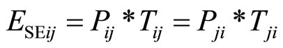
We model the transceiver as a finite state machine with two basic states (active and Sleep) and a transition state. Our energy model presents a typical radio transceiver of four active states, a sleep state (various degrees) and twelve transition states as shown in Table 1. To model the transceiver power consumption, we have simplified the actual power consumption characteristics with the assumption that power consumption occurs according to a symmetric and linear function within basic states i and when in transitions between two states i and j. The energy Ei consumed during a single visit to basic state i depends on the power consumption Pi of the underlying electronic circuitry and the time Ti spent in that state and is modeled as
 (2.1)
(2.1)
2.2. Active State
The active state is when transceiver is switch on and is ready for activities. Here the transceiver is sending or receiving data packets or in an idle state awaiting triggers from internal or external sources.
2.2.1. Transmit State
In transmit state; the transmitter electronics and amplifier consume large power to transmit data using the Friis free space equation in (2.6). Transmit state energy consumption model Etx is given as
 (2.2)
(2.2)
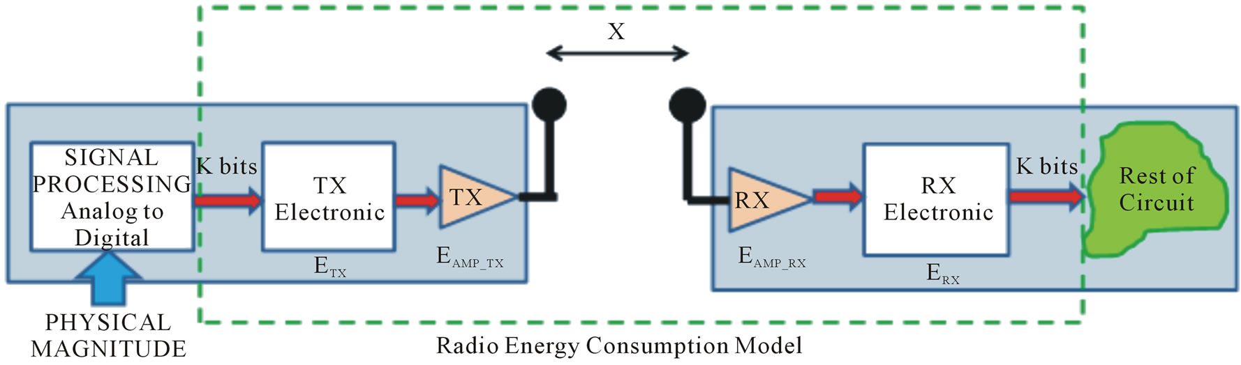
Figure 2. Block diagram of a typical transceiver [10].

Table 1. Transceiver states.
where transmit power Ptx is the sum of the transmitter electronics power overhead Poverhead and the amplifier power (PA) at transmit time Ttx.
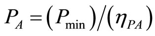 (2.3)
(2.3)
Ttx is also defined as the ratio of the number of bits (Nbit) and the bit rate (Rbit). Therefore Etx can be rewritten as:
 (2.4)
(2.4)
 (2.5)
(2.5)
 (2.6)
(2.6)
Pmin is the minimum power required for communication between two nodes at a distance d apart using frequency f. c is the speed of light 2.99 × 10⁸, n is the path loss, Gr, Gt are the antenna gain of receiver and transmitter respectively, where Rsens is the sensitivity of the receiver and LF is loss factor. Also the Header is the length of packet header, Payload is the length of packet payload, Trailer being the length of packet trailer and rate refers to the data rate.
2.2.2. Receive State
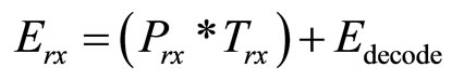
In this state, receiver is active and receiving data packet from the transmitter some distance away. We model the energy consumed when a receiver is active (Erx) as
 (2.7)
(2.7)
Prx and Trx are the power consumption of receiver electronic circuitry and the time duration respectively during data reception. Edecode is the energy required by the receiver to decode n bit of data packet.
2.2.3. Idle State
When a transceiver is active and ready but not currently receiving or transmitting data packets, it is said to be in an idle state. In this idle state, many parts of the transceiver circuitry are active, and others can be switched off. Most transceivers operating in idle state have power consumption almost equal to the power consumed in receive mode. The energy consumption in idle state Eidle is modeled as Etx and Er but in the absence of payload overhead or decoding cost as in Etx and Erx. For simplicity, we shall also model the Energy consumption of the receiver when sending beacon packets and doing clear channels assessment CCA as an idle state activity with beacon payloads overhead.
 (2.8)
(2.8)
Pidle is power used in this state listening to noise, doing a CCA scan or just nothing at time Tidle.
2.3. Sleep State
In the sleep state, a significant or all parts of the transceiver are switched off. There are transceivers offering several different sleep states, [1,15]. These sleep states differ in the amount of circuitry switched off and in the associated recovery times and startup energy [5,16]. For example, in a complete power down of the transceiver, the startup energy include a complete initialization as well as configuration of the radio, whereas in “lighter” sleep modes, the clock driving certain transceiver parts is throttled down while configuration and operational state is remembered. To get a complete energy consumption model for the transceiver, this energy consumption should also be factored into our calculation. Energy ESLP in sleep state is given as
 (2.9)
(2.9)
PSLP and TSLP is the power leaks of electronic circuits and time spent in sleep state.
2.4. Transition States
The power consumption during activation and de-activetion activities of electronic components for transitions between states i and j are different, though our simplified model assumes Pij = Pji and average power consumption is calculated as Pij ≈ Pi + Pj. The energy ESE consumed in transition state is modeled as
 (2.10)
2.5. Transceiver Energy Model
We present the Transceiver energy consumption as an aggregation of the energy consumption of the basic states (active and Sleep) and the transition states. From (2.2), (2.7), (2.8), (2.9) and (2.10), we present the transceiver energy consumption Etransc as
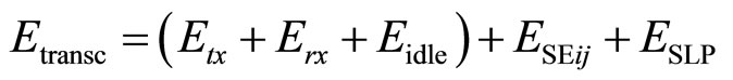 (2.11)
Our complete transceiver energy model is shown in Figure 3 as a finite state machine whose current state is de termine by an input or trigger which enables a state

Figure 3. Complete transceiver energy model.
transition. It models energy consumption in each basic state and transition.
3. Simulation Using Proposed Energy Model
Figure 4 shows the simulated transceiver energy consumption graph while transmitting data packets, listening, idle, receiving data packets and sleeping using our proposed model in an OPNET simulation environment. This simulated experiment evaluates the energy consumption tendency of the transceiver of a WSN node in different states using the energy consumption model abstracted in (2.12). In order to simulate and evaluate the transceiver energy model in OPNET simulation environment [17], we suppose a WSN node that consists of 5 Xbee-ZB-pro waspmote [15] from Libelium, acquiring temperature data from an aquacultural environment using a Unism digital temperature TH-10507 probe in a free space environment. The charged battery voltage (Vs) and current (Is) of Xbee-zb-pro waspmote are 4.2 V and 40 mA. Supposing the switch energy consumption of TH10507 are eoff-on = 0.0002 J and eon-off = 0.0001 J. We are assuming the energy consumption by the processor; sensor and other units remain constant within the duration of this simulated experiment. The node uses the random routing mode and the AODV routing protocol at a simulation distance of 100 m at a total time length of 200s.
In our experiment, we separated the energy consumption of the transmitter electronics from the energy consumption of the transmitter during data transmit. This is to emphasize the nominal contribution of the transceiver electronic components energy consumption to the total transceiver energy map and which is enormous. In the result of this simulated experiment as shown in Figure 4, the largest energy consumption is by electronic components of the transceiver, followed by the receive state. The power consumption by the electronic components’ like amplifiers, filters, ADC, DAC grows exponential with time therefore having the greatest impact on the energy trend curve. The energy consumption is lower in the idle states and transition states and is lowest during the Sleep state. There appears to be an inflection of the energy consumption curve of the various states at 140 ms, this could be as a result of attenuation of signal through the medium, consequently an increase in power uptake of the various states to compensate for path loss. This will form an interesting research topic in another paper and details are not covered here.
4. Transceiver Parameters of Consideration
From Equation (2.1)-(2.10), Figures 3 and 4 and Table 2, the range, frequency of transmission, antenna characteristics (sensitivity and gains), modulation and demodulation scheme, routing and MAC protocols, topology control, loss factor and data rate play important role towards the aggregate energy consumption map of a transceiver. This makes these parameters very important criteria points for consideration when designing a low power WSN.
There are several factors that affect the power consumption characteristics of a transceiver radio [18,19]. Radio state,

Table 2. Transceiver modules in Libelium Waspmotes [15].
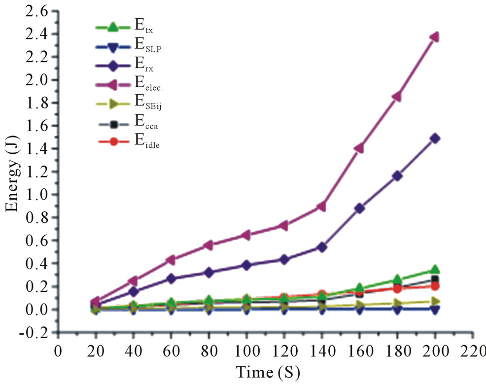
Figure 4. Transceiver States energy consumption.
duty cycling, transmission power and message sending rate are considered as factors that affect the average power consumption of a node [20]. A sensor node draws different levels of power depending on its transceiver states of transmission; sleep, transition or awake states. Also the average energy consumption of a sensor node changes depending on desired range of transmission and rate of data transmission. Designing low power WSN will require minimizing power consumption in different transmission states, rates of data transmission and range of transmission.
4.1. Transmission Range
The range of transmission of a wireless sensor node is controlled by several factors. A relationship exist between the range of transmission of a transceiver, radiated power of a transceiver, frequency of transmission, antenna gain, receiver sensitivity and the loss factor as shown in the Friis Equation (2.1) [19,21].
The most intuitive factor is that of radiated power for inter-node communication between two nodes. From (2.1), the further the distance a transmitting node is from the receiving node, the more power amplification needed for data transmission. For a low power design, it is necessary to locate the nodes in a network close to each other and make use of a multi-hop transmission scheme from the source node to the sink. In Table 2, the transmitting distance of 500 m on 2.4 Hz frequency consumes only 1 mW, while achieving the distance of 7000 m on the same frequency consumes 50 mW. So, minimizing distance between nodes will also minimize the power expenditure of the transceiver as the farther the inter node communication, the more energy required to make the signal travel.
Other factors in determining transmission range and power consumption include choice of frequency, the sensitivity of the receiver, the gain and efficiency of the antenna and the channel encoding mechanism.
Lower frequencies suffer less path loss and better range than higher frequencies, although higher frequencies result in smaller sensor nodes [22].
The communication range or distance will be greatly extended when using lower frequencies due to low path loss attenuation. With low path propagation loss, the antenna gain would not become an important factor in the system link budget. Communication using lower frequencies would be an ideal choice if the density of deployment of a WSN allows for some short distances apart between nodes. Multi-hop, short-range inter nodal communication can also be adopted so that more nodes can be in the network to reduce power consumption as this also decrease the single-hop communication distance. Table 2 shows the transceiver characteristics of Libelium motes. On the same transmit power of 100 mW and antenna sensitivity of approximately 100 dBm; the transceiver using the 900 Mhz frequency is able to cover a distance of 12 km while the transceiver on 2.4Ghz is just able to cover 7 km. It is also clear that while transmitting on the same frequency of 2.4 GHz, the same distance of 7 km is still achieved with 50% of the transmitting power.
This is achieved by a 3 dBm improvement of the sensitivity of the antenna. Such an improvement allows reducing the transmit power which prolongs the lifetime of the node. Hence, increased transmission range is achieved by either increasing sensitivity or by increasing radiated power.
In general, wireless sensor network nodes cannot exploit high gain, directional antennas because they require special alignment and prevent ad-hoc network topologies. Omni-directional antennas are preferred in ad-hoc networks because they allow nodes to effectively communicate in all directions. For WSN applications, an isotropic antenna (Gr and Gt =1) is desired as the relative orientation between sensors nodes are not predetermined. Also, multi-path is more severe in indoor environment and the path loss exponent n is typically between 3 and 4 [19,22].
4.2. Transmission Rates
Several parameters play important role in the transmission data rate of the transceiver. Chiefly amongst them are the modulation scheme chosen for implementation, the desired data throughput, the MAC protocol and the topology of the network.
4.2.1. Modulation
[23] present several modulation schemes suitable for use in designing low power WSN such as frequency shift keying (FSK), Gaussian minimum-shift keying MSK, Quadrature phase shift keying (QPSK, OQPSK, π/4- QPSK). The spectrum efficiency of MSK is higher than FSK, but the demodulation is more complex and frequency hopping cannot be realized for MSK. Since power consumption is a design constraint, power-efficient modulation such as binary frequency-shift keying (BFSK) could be a good candidate for a WSN [22]. The ability of Binary phase shift keying BPSK to avoid interferences is better than that of FSK; and OQPSK is more spectrally efficient. But the demodulation circuits of both BPSK and offset quadrature phase-shift keying (OQPSK) are complex and ADCs are usually needed and not recommended for applications of low data rates. With lower data rate, simpler modulation schemes such as on-off keying (OOK) and frequency shift keying (FSK) can be employed. These schemes allow the use of the less complex direct modulation transmitter. However, in applications that have a high data rate and a strict spectrum limitation, MSK, BPSK, O-QPSK and even OFDM can be adopted.
4.2.2. Data Rate
In typical deployment, data of interest vary slowly with time, thus, to achieve sensor network for these applications, a data rate of only hundreds to thousands of bits per second is sufficient. For low power consumption, the oscillator start-up time is long, which seriously restricts the data rate of an OOK system. Therefore the traditional OOK transmitter is often used in low data rate applications of less than few Mbps. Methods have been proposed to increase the data rate with low power OOK system as the transceiver operates at a higher instantaneous data rate and turn off the radio periodically [14]. However, there is an upper limit above which increased duty cycling and higher instantaneous data rates decrease energy efficiency. One key problem is that the start-up time associated with turning on a transceiver has an associated energy that cannot be reduced by increasing data rates [15]. As alternative method for higher data rate in an OOK transceiver is based on the mixer-based frequency up-conversion transmitter, but it is not suitable to realize low power consumption and compact size. Therefore, a transceiver architecture that meets the requirements of wireless sensor networks must be carefully chosen.
4.2.3. Protocols
Inefficient MAC consumes alot of its energy to monitor channel. In low power MACs radios are set on either pre-scheduled times or asynchronous in need basis [11]. This reduction in duty cycle can be seen directly in battery lifetime. MAC protocols must avoid collisions due to simultaneous transmissions and must perform other important functions like addressing, error checking and delivery notification. An efficient MAC protocol should possess many characteristics.
4.3. Transmission States
From Figure 4, the energy consumption of a WSN node varies according to the state of the transceiver with energy consumption being highest in the electronic component, followed by the receiving state, and lowest in the sleep state. Achieving low power design will require sensor nodes to be in perpetual state of sleep (if possible) where power consumption is lowest or to duty cycle between active state and sleep state. In duty cycling to reduce the transceiver power consumption, the objective is to minimize time spent in the active states and transition states.
One of the ways to minimize transceiver time spent in active states is to transmit at a high data rate and quickly switch back to sleep state. However transmitting at high data rate requires a higher transmit power to achieve the same bit error rate and increases the receiver power due to tighter constraints on timing recovery, higher analogto-digital (A/D) sampling rate, and possibly more complex modulation schemes. Transmitting at low data rate will implies longer time in transition between states and cumulative energy consumption in transition state could be enormous making it unnecessary to change state from active state to sleep state.
We can overcome these challenges by processing data locally within the node and transmitting or forwarding only aggregated or compact data to the receiving node since power consumption by the processor is lower than the transceiver [1]. Also to achieve a short transition time, the frequency synthesizer and operating points of the circuits must be designed to settle to their steady-state value quickly [22]
5. Conclusion
Energy consumption as discussed in this paper is a precious resource in wireless sensor networks. Considerable energy efficiency should make an evident optimization goal and be carefully distinguished to form actual, measurable figures of merit. Understanding and applying the transceiver energy consumption models abstracted here will enable design of an efficient and low power WSN as energy consumption parameters are often inter related with performance and other user expectations.
REFERENCES
- Holger Karl, and Andreas Willig,’’Protocols and Architectures for Wireless Sensor Networks. John Wiley & Sons, 2005, pp. 15-329. doi:10.1002/0470095121
- C.-Y. Chong and S. Kumar,"Sensor networks: Evolution, opportunities, and challenges", Proc. IEEE, Vol. 91, No. 8, pp.1247-1256, 2003. doi:10.1109/JPROC.2003.814918
- A. Chandrakasan, R.Min, M. Bhardwaj, S-H Cho, and A.Wang, “Power Aware Wireless Microsensor Systems,” ESSCIRC, Florence, Italy, September 2002 .
- I.F. Akyilm diz et al., “Wireless Sensor Networks: A Survey,” Computer Networks, vol. 38, 2002, pp. 393-42.
- J. Moreno Molina, J. Haase, C. Grimm and J. Wenninger “Energy Profiling Technique for Network-Level Energy Optimization” IEEE Africon 2011 - The Falls Resort and Conference Centre, Livingstone, Zambia, 13 - 15 September 2011 doi:10.1109/AFRCON.2011.6072073
- Ali Norouzi and Ahmet Sertbas, “An Integrated Survey in Efficient Energy Management for WSN using Architecture Approach“, Int. J. Advanced Networking and Applications Volume; 03, Issue; 01, Pages: 968-977 (2011).
- Vikas Kumar and Rajender Kumar” Low Power Wake up Receiver for Wireless Sensor Network” IJCST Vo l. 1, IS Su e 1, Se p t. 2010.
- A Roy and N Sarma, “Energy Saving in MAC Layer of Wireless Sensor Networks: a Survey” “National Workshop in Design and Analysis of Algorithm (NWDAA)”, Tezpur University, India, 2010”.
- Jerker Delsing, John Borg, Jonny Johansson” Architecture for Extreme Low Power Sensing in Wireless Sensor Network Devices”: The Fifth International Conference on Sensor Technologies and Applications, SENSORCOMM 2011.
- Sandra Sendra, Jaime Lloret, Miguel García and José F. Toledo.“Power saving and energy optimization techniques for Wireless Sensor Networks“, Journal of communications, Vol 6. No 6, Sept, 2011.
- B. Han, D. Z. Zhang and T. Yang, “Energy Consumption Analysis and Energy Management Strategy for Sensor Node, ”International Conference on Information and Automation, Proceedings of the 2008 IEEE, Vol. 6, 2008, pp. 211-214.
- Q. Yang, X. H. Chen and J. H. Shi, “Low Power Design of the Terminal Node for Wireless Sensor Network,” Journal of Xiamen University (Natural Science), Vol. 47, No. 3, 2008, pp. 357-358.
- X. F. Wang, J. Xiang and B. J. Hu, “Evaluation and Improvement of an Energy Model for Wireless Sensor Networks,” Chinese Journal of Sensors and Actustors, Vol. 22, No. 9, 2009, pp. 1319-1321.
- Wikipedia, “Finite State Machines”. http://en.wikipedia.org/wiki/finite_automata.
- Libelium Corporation,“Waspmote Technical guide”. December, 2011, http://www.libelium.com /documentation/waspmote/waspmote-technical_ guide_ eng.pdf.
- J. Moreno Molina, J. Haase, and C. Grimm. “Energy consumption estimation and profiling in wireless sensor networks. In ARCS ’10 - 23th International Conference on Architecture of Computing Systens 2010 Workshop Proceedings, pages 259–264, Feb. 2010.
- X. Li, “Network Modeling and Simulation with OPNET Modeler,” Xidian University Press, Xi’an, 2006, pp.1-15.
- The Friis Equarion: http://www.antenna–theory .com/basics/friis.php. Accessed: February 15th, 2012.
- Atmel, ‘’Range Calculation for 300 MHz to 1000 MHz Communication Systems’’ http://www. Atmel.com/ Images/doc9144.pdf. February 16th, 2012.
- James A. Anderson and Thomas J. Head, “Automata theory with modern applications.” Cambridge University Press. pp.105–108. (2006) ,ISBN9780521848879.
- Rappaport, T. S., Wireless Communications: Principle and Practice. Prentice Hall, 2nd Edition, 2002.
- Roshdy Hafez,Ibrahim Haroun,Ioannis Lambadaris ’’Building Wireless Sensor Networks’’ED Online ID#11071,Sept,2005 .http://mwrf.com/Article/ ArticleID /11071/11071.html, Accessed :January, 2012.
- Bo Zhao and Huazhong Yang .“Design of Radio-Frequency Transceivers for Wireless Sensor Networks”, http://www.intechopen.com/source /pdfs/12477/InTech-Design_of_radio_frequency_transceivers_for_wireless_sensor_networks.pdf. Accessed: January, 2012.