Wireless Sensor Network
Vol. 5 No. 7 (2013) , Article ID: 34311 , 13 pages DOI:10.4236/wsn.2013.57017
COCM: Class Based Optimized Congestion Management Protocol for Healthcare Wireless Sensor Networks
1Department of Computer Engineering, Science and Research Branch, Islamic Azad University, Tehran, Iran
2Department of Computer Engineering, Ferdowsi University of Mashhad, Mashhad, Iran
Email: aa.rezaee@srbiau.ac.ir, hyaghmae@ferdowsi.um.ac.ir, Rahmani@srbiau.ac.ir
Copyright © 2013 Abbas Ali Rezaee et al. This is an open access article distributed under the Creative Commons Attribution License, which permits unrestricted use, distribution, and reproduction in any medium, provided the original work is properly cited.
Received May 17, 2013; revised June 16, 2013; accepted June 30, 2013
Keywords: Wireless Sensor Networks; Active Queue Management; Congestion Control; Healthcare; Multi Path Routing
ABSTRACT
Wireless Sensor Networks (WSNs) consist of numerous sensor nodes which can be used in many new emerging applications like healthcare. One of the major challenges in healthcare environments is to manage congestion, because in applications, such as medical emergencies or patients remote monitoring, transmitted data is important and critical. So it is essential in the first place to avoid congestion as much as possible and in cases when congestion avoidance is not possible, to control the congestion. In this paper, a class based congestion management protocol has been proposed for healthcare applications. We distinguish between sensitive, non-sensitive and control traffics, and service the input traffics based on their priority and quality of service requirements (QoS). The proposed protocol which is called COCM avoids congestion in the first step using multipath routing. The proposed AQM algorithm uses separate virtual queue's condition on a single physical queue to accept or drop the incoming packets. In cases where input traffic rate increases and congestion cannot be avoided, it mitigates congestion by using an optimized congestion control algorithm. This paper deals with parameters like end to end delay, packet loss, energy consumption, lifetime and fairness which are important in healthcare applications. The performance of COCM was evaluated using the OPNET simulator. Simulation results indicated that COCM achieves its goals.
1. Introduction
Wireless Sensor Networks (WSNs) are one of the most important technologies that have been improved due to recent developments in wireless communication and are applied in different areas such as healthcare applications [1-4] . They have inherent characteristics unlike traditional wireless networks. Sensor nodes have scarce resources for computation, storage, communication bandwidth, and, most importantly, energy supply. Recently, extensive studies have been done in different layers of WSN’s [5,6] . The event-driven nature of WSNs leads to unpredictable network load, especially in healthcare applications. Typically, WSNs carry the low traffic load when there are no special events. But the occurrence of important events may cause a burst traffics which leads to congestion in the network. Transport protocols control congestion in end to end or cross layer manner.
Nowadays, Healthcare Wireless Sensor Networks have received great attention due to the properties of WSNs such as reliability, interoperability, efficiency, low-power consumption and inexpensiveness. One of the applications of WSNs is remote monitoring of patients by doctors and nurses which eliminates the need to be physically present in the patient sites [7]. Figure 1 shows different sensors attached to patients which are capable of sensing patient information which can be sensitive (vital signs, such as the heart rate and breathing condition) or non-sensitive (motion signs, such as leg sensors). The received information can be transmitted to the control center with the help of a PDA and neighboring nodes. Sensitive information needs low delay and low packet loss while non-sensitive data can tolerate more delay and more packet loss. We restricted ourselves to healthcare applications which require stationary sensor nodes (they do not change their locations for at least a few hours).
In medical emergencies, it is quite likely that the sensors placed in the different patients, sense and transmit vital patient information very frequently and simultane-
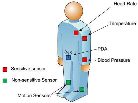
Figure 1. Type of sensors on a person body.
ously. This leads to increased likelihood of network congestion in such applications. Congestion in WSNs leads to dropping of packets at the nodes, increased consumption of the limited energy in the nodes and reduction of the throughput of the network. In life-critical applications involving large numbers of patients, congestion is extremely undesirable and may lead to the death of a patient. However, timely arrival of the packets at their destinations ensures the safety and survival of the patients. Obviously, complete elimination of congestion is unlikely. But, it’s possible to significantly reduce the effects of congestion, i.e., significantly decreasing the number of packets that get dropped due to congestion, the large amount of unwanted consumption of the limited energy at the sensors and increasing the number of packets that get successfully delivered with respect to the number of packets which are sent from the different nodes.
We addressed the problem of congestion by proposing a new approach to avoid it. In this approach, congestion will be avoided by distributing packets through multiple routes and if congestion still occurs, we run an optimized congestion control algorithm.
Congestion control algorithms are classified as source based or network based. Source based algorithms are deployed at the end host where the transport protocol is responsible for detecting congestion in the network. Network based algorithms, on the other hand, are implemented in the intermediate network devices, especially routers. Based on the degree of congestion detected in the network, source based algorithms adapt the rate at which the application is sending traffic. This mechanism, more popularly known as end to end congestion control is employed by transport protocols such as the Transmission Control Protocol (TCP). In network based algorithms, the intermediate network equipments are responsible for detecting oncoming as well as subsisting congestion and provide feedback to the sender for indicating the situation. Source based algorithms work well for traffic that is responsive to congestion e.g. TCP traffic. However, non-sensitive traffic e.g. User Datagram Protocol (UDP) traffic may still cause congestion due to its greedy behavior. Thus, the need arises for network based congestion avoidance and control mechanisms.
Basically, two factors cause congestion in sensor networks (see Figure 2). The first is when the packet arrival rate is higher than packet service rate which occurs mostly in nodes closer to the sink. The second is the performance at the link level including competition, collision and bit error. This type of congestion occurs on the link.
In this paper, we have proposed a new congestion management protocol for healthcare application in wireless sensor networks. Proposed protocol is composed of two main parts, routing and congestion control. Proposed routing protocol is a data centric protocol which composed of 4 different phases. The phases are discussed in Section 3 in details. We have evaluated the requirements of the healthcare applications, and consider them in designing proposed protocol. Forth phase of proposed routing protocol is data transmission. Similar to other networks, congestion may occur in network nodes. We have also proposed a congestion control mechanism which is discussed in Section 3.4. As its main job, congestion control mechanism adjusts nodes sending rate (especially source nodes) in order to manage congestion in intermediate nodes. In Section 4, simulation results have been presented. And finally in Section 5, we conclude the paper.
2. Related Works
Different protocols have been proposed for congestion control. These protocols are different in terms of congestion detection, congestion notification, and rate adjustment mechanisms (Table 1). Congestion detection methods that are employed in Wireless Sensor Networks may use queue length [8-12] , packet service time [13], the ratio between service time and packets inter-arrival time [14], Packet service ratio [15] or dual buffer thresholds and weighted buffer difference [16]. For sensor networks using MAC layer protocols such as CSMA, channel load
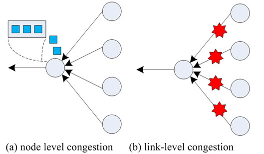
Figure 2. Type of sensors on a person body.
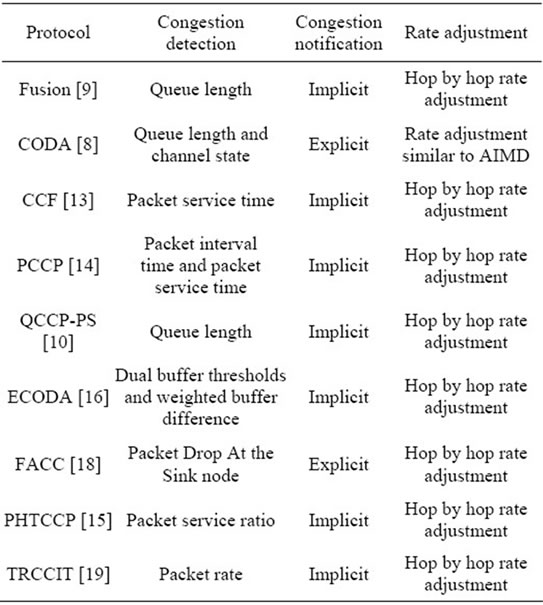
Table 1.Congestion control protocols for WSN.
can also be used as a tool for congestion detection [8]. When congestion is detected, transport protocols notify congestion information from the congested nodes to other nodes on the route to the sink or the source nodes. Congestion information can be as small as a binary Congestion Notification (CN) bit [8,9] or contain more information such as permitted data rate [13] or congestion degree as in [14]. Sensor nodes can adjust their sending rate after receiving congestion notification. If a bit CN is received, the Additive Increase and Multiplicative Decrease (AIMD) method or other types of it are applied. However, if more comprehensive congestion information is available, rate adjustment can be done more accurately.
Congestion control and fairness protocol (CCF) [13] detects congestion based on packet service time. The CCF method carries out upstream congestion control using a scalable and distributed algorithm that ensures the fair delivery of the packets to the central station as well as removing congestion. CCF formulates congestion control and determines the number of downstream nodes, the average sending rate of the packets and the production rate in each sensor. Priority-based Congestion Control (PCCP) [14] is a priority based upstream congestion control protocol and measures a congestion degree as the ratio between packet arrivals and packet service time. PCCP also uses a rate adjustment algorithm unlike that of the AIMD technique. It supports fairness in weighted sensor nodes. PCCP uses different degrees of priority indexes, so a sensor node with a higher priority index uses more bandwidth and injects more traffic. PCCP allows the application layer to cancel the priority index in a special area in each senor node. This aspect can be useful for a large number of sensor network applications. There are limitations for PCCP which include the lack of packet recovery. Queue based Congestion Control Protocol with Priority Support (QCCP-PS) [10] is a queue based Congestion Control Protocol with Priority Support which uses the queue length as a congestion degree indicator. It controls the congestion with the packet priority based on the node priority for a WSN. QCCP-PS also improves the PCCP by controlling the queue more finely but it does not have any mechanism for handling prioritized heterogeneous traffic in the network. The sending rate of each traffic source in the QCCP-PS is increased or decreased based on its congestion degree and its priority index. The rate adjustment for each traffic source is based on its priority index as well as its current congestion degree.
Enhanced congestion detection and avoidance (ECODA) [16] uses dual buffer thresholds and weighted buffer difference for congestion detection. This method is different from traditional single buffer threshold methods [8,13,14] . It can differentiate congestion level and dealt with them correspondingly. ECODA is composed of three mechanisms: 1) Using dual buffer thresholds and weighted buffer difference for congestion detection; 2) Flexible Queue Scheduler based on packet priority; 3) A bottleneck-node-based source sending rate control scheme in case of persistent congestion. ECODA also adopts hop-by-hop congestion control scheme for transient congestion.
Fuzzy congestion controller for wireless sensor networks (FCC) [17] develops a fuzzy rule base as well as fellowship functions. It uses channel load and queue size of intermediate nodes as the indication of congestion to organize the inputs. The output is branched from the fuzzy rule base and the fuzzy reference engine conjuncts and determines new source rates. This algorithm reduces packet loss comparing with non-fuzzy methods. It increases throughput and energy consumption.
3. The Proposed Protocol
The proposed protocol has been designed for congestion management in Wireless Sensor Networks for healthcare applications. The main objective of the proposed protocol is to avoid, or if not possible, control congestion in Wireless Sensor Networks. Similar to other data centric protocols such as reliable and energy efficient protocol (REEP) [20] and Directed Diffusion (DD) [21] and our previous work [22] has been developed in different phases. These protocols use different phases to perform different crucial tasks. COCM considers two main parameters, energy and delay (besides lifetime and fairness). In all routing protocols which are developed for WSNenergy should be considered as a goal parameter. In healthcare applications delay is the main goal parameter. COCM considers two types of traffics: Sensitive and Non sensitive. Sensitive traffics are designed to transfer high priority data (they need low delay) and Non sensitive traffic is designed to transfer normal traffic.
The proposed protocol works in the following phases:1) request dissemination which is performed by the sink, 2) event occurrence report which is performed using packets that are forwarded from sensors located on the patients body to the sink, 3) route establishment, 4) data forwarding and rate adjustment in case of congestion occurrence. In the design of COCM, congestion control as the main objective affects other objectives. Routing has been considered as a part of the general objective. In this protocol, data are sent with different priorities. Therefore it can be used for healthcare remote monitoring applications whose networks contain data with different levels of importance and different priorities for different patients.
The proposed protocol acts as a cross layer. As mentioned before, in COCM the duties of transport layers and the network are carried out simultaneously. First, the sink (the telemedicine center) sends its requirements (required information) to network nodes (sensors connected to the patient’s body). In the meantime, any network node observing the event specified by the sink, will inform the sink with an event report (patient’s condition) using the phase 2 procedure. In the second phase, the initial routing tables are formed. These tables are then used in the third phase where different routes are chosen in the final routing tables. The final tables are produced in the third phase depending on the priority of the transferred data.
The fourth phase is the data forwarding phase in which the data recorded from the events observed by nodes are given to the sink. A large volume of data is moved in this phase; therefore a procedure for congestion control is needed. In COCM, an adaptive procedure has been proposed for controlling source sending rates. This procedure is also carried out in the fourth phase in case of congestion.
Generally Figures 3-5 show the proposed protocol structure.
3.1. Request Dissemination Phase
This is the first phase in carrying out the routing protocol. In this phase, information required by the sink node (medical center) such as patients’ vital signs should be sent to all network nodes. In other words, sink requirements are requested and distributed throughout the network based on different algorithms presented for distributing data in Wireless Sensor Networks. However, the type of data is very important. In some situations, pa-
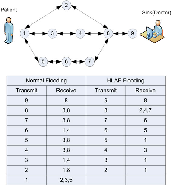
Figure 3. Request Dissemination Phase.
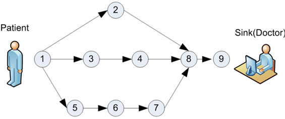
Figure 4. Event Report Phase.
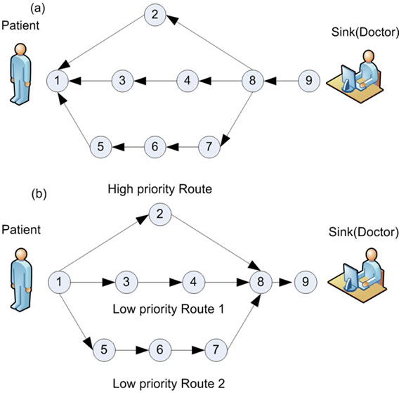
Figure 5. (a) Route Establishment Phase (b) Data Forwarding Phase.
rameters may include highly sensitive information such as heartbeat or blood sugar level (for some patients such as those with diabetes). The accepted values for different parameters are determined by the expert.
This phase is started with the sink and the packets that are used for the implementation of this phase have the same structure. The proposed protocol uses a healthcare aware location aided flooding (HLAF) algorithm in this phase. HLAF is designed on basis of LAF [23]. LAF protocol is designed for Wireless Sensor Networks and it is not efficient enough for healthcare applications.
In HLAF we consider network as a virtual grid. In healthcare applications the network nodes (patients) are aware of their own geographical position. Considering network’s boundary we can simply form virtual grid. For instance if a 200 × 200 bounded network needs a 64 cell grid, cells with 25 × 25 bounded will be formed. Each node can find its own cell knowing its geographical position and width of grid cells. We define two types of nodes in each cell. Nodes with all their neighbors inside its own cell are called internal nodes, and those with at least one neighbor in another cell are entitled as edge nodes. Each HLAF packet has a field in which list of visited node IDs are saved. By the time each node intends to send a packet to its neighbors, it stores their IDs in the mentioned field. Each node evaluates this field after receiving a packet. If it finds its ID in the list, it will drop the packet; otherwise it forwards the packet to its neighbors, as mentioned above. By this routine, the number of forwarded redundant packets and energy consumption decreases.
This algorithm supports distribution of data with different priorities which is useful for healthcare applications like medical monitoring in which data distribution depends on the position of the target nodes (patients).
3.2. Event Report Phase
After the request dissemination phase, if a sensor senses an event based on its duty, it will report the sign to the sink according to the specifications. The report must have the required characteristics so that the sink can show the proper reaction.
In this phase, the information related to the occurring event is sent to the sink, however basic data related to the event are sent in the data forwarding phase. Moreover, the preliminaries of packet routing are also determined in this phase. For this purpose, the patient node creates a packet containing the information related to the sensed event and sends it to all its neighbors. Since nodes (patients) are aware of their own positions the packets are sent to the neighbors that are closer to the sink than the sender. The routing tables required for the routing of node data in the route from the packet to the sink will be provided. And the final routing will be carried out in the route forming phase.
After creating the packet (which we call phase 2 packet), if the nodes are aware of their positions this will lead to lower energy consumption for the protocol. However since we need to locate all the nodes it cannot be applied everywhere. It is worth noting that in applications where the request should only be sent to part of the network, nodes are aware of their positions.
After receiving the packet from phase 2, each node creates a record labeled phase 2 table in a routing table. The priority of the packet (compared to the priority of the traffic and the event in question), the source node, the sender, the length of the covered route and the number of covered hops are kept in this record. In the proposed protocol, each node has an ID that is placed in all outgoing packets. The length of the covered route is obtained from the length of the route from the source of the packet to the current node. After creating the record, the node sends the packet back to its neighbors. This procedure is repeated until the packet reaches the sink.
Keep in mind that from any source, there could be more than one record in each node’s phase 2 table. The reason for this is that phase 2 packets may arrive at a node from different routes. Only packets with identical fields are ignored.
At the end of phase 2, each node has a routing table called phase 2 table which is used for final routing in phase 3. Records in phase 2 routing table determine the possible routes between the desired node and the source node sensing the event.
3.3. Route Establishment Phase
After the arrival of phase 2 packets at the sink, a type 3 confirmation packet is sent to the source node by the sink which notifies the source node to send its data to the sink for processing. Then, sensors from one or more patient(s) may send messages. In this stage, the sink chooses one or several nodes for the final transfer of data based on the information sent from source nodes. In phase 2 packets, each node specifies the level of its importance. For example, the heart beat sensor or the kinesthetic sensor connected to the patient’s foot sends a message to the center and specifies the level of importance. The sink chooses the source node for the patient’s report based on the specified level of importance.
Following the selection of the source, phase 3 packets are sent. As the phase 3 packet moves along the route, it creates a phase 3 routing table. Phase 3 routing table is the final routing table for routing the data sent from the source. The transfer confirmation depends on the priority of the sensed event. Two types of confirmations are considered, high priority confirmation (sensitive traffic) and low priority confirmation (non-sensitive traffic).
The sink checks the phase 2 routing table in order to send a high priority confirmation. The first record is chosen for sending confirmation. Phase 2 packets are then arranged chronologically in the phase 2 routing. Upon receiving a type 2 packet, the nodes place it in the first record. In fact, the number assigned to the packet record in the phase 2 routing table determines their time sequence. Since time is very important in sensitive applications, the first record in the phase 2 routing table which is chronologically the first created record is chosen. However, in choosing records, the source node in the record is always considered. Moreover, only records in which the source node is the one chosen by the sink will be considered.
Each node forms two tables in phase 3: Phase 3 routing table with high priority and phase 3 routing table with low priority. During this phase, two tables are completed. Routing table of each node maintains the best routes to the sink through its neighbors which are closer to the sink. Considering the maximum number of neighbors for each node in WSN, the routing table will be practical and small.
When a node receives a phase 3 packet with high priority, it creates a high priority record for the packet in the phase 3 routing table. This table consists of the following components: sender (the source node of the receiving phase 3 packet with high priority), receiver (the destination node for the phase 3 packet with high priority), source node (the node sensing the event which is the final destination of the phase 3 packet) and type of application (this component will be used in networks designed for multiple applications). Based on what has been mentioned so far, each node chooses the first record from the phase 2 routing table as the next hop for the high priority phase 3 packets. This procedure will continue until the packet reaches the source. In fact, at the end of phase 3, a record is placed in the sensitive phase 3 routing table for each source.
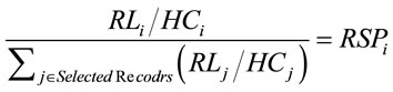
What has so far been mentioned in Section 3.3 is related to high priority traffic. We will go on to explain the creation of low priority phase 3 routing table. From among the records in the phase 2 routing table, the sink considers the records chosen in relation to the source. For each of these records, the probability RSPi is computed using Equation (1).
 (1)
(1)
where RLi is the route length between node i and the sink and HCi is the hop count for the ith record route. RSPi is the Route Selection Probability of choosing the record as the next hop for the low priority phase 3 packets. After determining RSPis for all the records with the intended source, two records are chosen based on probability. Then, the low priority phase 3 packet is sent to these records. Different routes are chosen so that fairness is observed in energy consumption of the network nodes.
Each node receives a phase 3 packet with low priority and records it in its routing table. Then, through a procedure similar to that of the sink, the next two neighboring hop neighbors are chosen and the phase 3 packet is sent to them. All the characteristics are recorded in non-sensitive phase 3 routing records.
3.4. Data Forwarding Phase
Towards the end of phase 3, sensitive and non-sensitive phase 3 routing tables are created. Each node will contain a sensitive phase 3 routing table and a non-sensitive phase 3 routing table. This provides multipath routing for our proposed protocol and can distribute packets through more than one path.
Depending on the type of the sensed event, the source node can send its data to the sink after receiving sensitive traffic from phase 3. As mentioned before, all nodes including the source node have two types of routing table. Sensitive phase 3 routing table is used for sending sensitive data and non-sensitive phase 3 routing table is used for sending non-sensitive data.
In the sensitive phase 3 routing table, there is only one record toward the sink for each source. Each node receives sensitive traffic from the node in question and uses the traffic to send the record to the next hop. However, in each non-sensitive phase 3 routing table, there will be more than one record for each source in the table. Each record has a probability RSPi based on which the next hop is chosen. The greater the RSPi in the record, the more likely it will be chosen. Finally, a record will be chosen as the next hop and data are sent to this record.
Congestion Control Mechanism in Inter-Mediate Nodes
Our goal is to provide routing and congestion management in WSN’s for healthcare applications. Congestion management comprises two phases. Congestion avoidance and congestion control. Congestion avoidance is implemented with distributed routing algorithm (Section 3).
AQM schemes are one of the important mechanisms that provide quality of service and prevent congestion in IP networks that perform special operations in our protocol to achieve better performance for end flows [24]. With these mechanisms, congestion is controlled and network degradation is avoided [25]. Figure 6 depicts the queuing model on an intermediate node. In this figure a classifier has been provisioned in network layer. The purpose of a classifier is to classify different types of data and route them in their corresponding queues. The type of data is located in the packet header. We define three types of traffic; high priority (HP), low priority
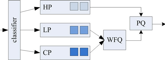
Figure 6. Per class queuing in the intermediate sensor node.
(LP) and control packets (CP). Sensitive traffics are sent to class 1, non-sensitive traffic sent to class 2 and control packets are sent to class 3.
In our proposed protocol we use the Weighted Fair Queuing (WFQ) scheduler to guarantee fairness between different traffic classes. We also use Priority Queue (PQ) for high priority traffic. The use of PQ ensures low latency and more reliability for sensitive traffics. PQ allows sensitive traffics to be serviced and sent first. While there is a class1 packet in the queue, the scheduler sends class1 packets the queue. In order to provide fairnessbetween class 1 and other classes, only 20 percent of network bandwidth is assigned to class1 traffics, so using PQ scheduler does not cause unfairness.
1) Proposed AQM COCM uses a flexible procedure for queue management.
Pi is the packet loss probability which is determined by an Active Queue Management (AQM) mechanism. The proposed procedure shares the queue in each node for the flows passing the node. However, the boundaries between queues are not fixed; meaning that if one of the active flows has free space in its queue, other flows facing a lack of space can use this free space on certain conditions. In other words, queues in Figure 6, are separated virtually with flexible boundaries.
The probability of the drop (Pi) of a packet in ith queue is determined using the following Equation (2).
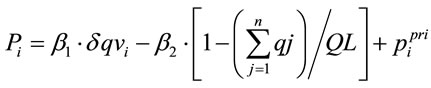 (2)
(2)
When a packet is received by the node, drop probability Pi is computed for the packet. Packet will be queued or dropped, based on Pi value. In fact, higher probabilities of loss for a flow show that the corresponding queue is in critical status with respect to the congestion. Therefore, the weight of Pi has been used directly in determining the sending rate and the degree of congestion in each node. The process of finding Pi is performed locally in each node.  is an initial value for Pi which is determined using Equation 3. qj presents the number of packets stored in jth virtual queue. dqvi shows the level of variation in the length of the ith virtual queue. The value of dqvi can be positive or negative. dqvi is multiplied by coefficient b1 as presented in Equation 4. If dqvi is positive, it will remain positive after multiplying by b1 and will finally cause an increase in Pi. It means that if the variation in the flow queue length is positive (the queue size is prolonged) the packet loss probability and the probability of congestion are increased. b2 specifies the flexibility of the flow queues. The expression
 ![]() specifies the total used space in the node queue. Dividing the total by QL (total space in the node queue) gives us the percentage of used space in the node queue. Multiplying this value by b2 will result in a number which reduces the value of Pi. In other words, the greater the free space in the queue the lesser the packet loss probability of the flows. However, the effect of this value depends on the b2 parameter. b1 and b2 are determined based on node priority by the user.
specifies the total used space in the node queue. Dividing the total by QL (total space in the node queue) gives us the percentage of used space in the node queue. Multiplying this value by b2 will result in a number which reduces the value of Pi. In other words, the greater the free space in the queue the lesser the packet loss probability of the flows. However, the effect of this value depends on the b2 parameter. b1 and b2 are determined based on node priority by the user.
 (3)
(3)
 (4)
(4)
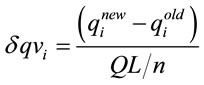
The parameters in Equations (2)-(4) are determined in a periodical manner. Therefore, in Equation (4) the value of  is the queue length in the ith flow in the preceding calculation and the value of
  is the queue length in the ith flow in the present calculation. Generally, in all the equations qi shows the queue length in the ith flow. Parameter n is the number of node’s neighbors.
2) Proposed Rate Adjustment Congestion control, as mentioned in Section 1, consists of two parts: a) congestion notification, and b) rate adjustment. These procedures are done interestedly in a hop by hop manner, from the congested node to the source node with rate adjusting packets including children rate portions. As discussed in Section 3.4, AQM considers arrival rate 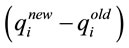 and queue length (q) in order to determine Pi. We use Pi as congestion indicator. Following using proposed optimization problem (Equations (5)) the upstream neighbor’s rate adjustment is performed.
Since data are transferred in the data forwarding phase, it is likely to have network congestion in this phase. COCM controls congestion by controlling the sender’s data sending rate. However, congestion will also be prevented as far as possible, using multiple routing. The mechanism of congestion control comprises two parts: active queue mechanism in intermediate nodes and sender rate control mechanism. Active queue mechanism manages queues as well as detecting the level of congestion.
The following equations show the optimization problem which is used in order to control the forwarding rate.
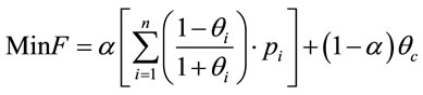 (5-1)
(5-1)
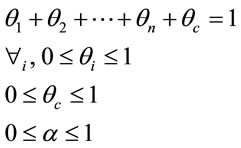 (5-2)
(5-2)
 (5-3)
(5-3)
In Equation (5-1), n is the number of upstream neighbors and Pi is the drop probability computed by Equation (2). The aim of optimization is to minimize the function of Equation (5-1). Figure 7 clarifies the variables in Equations 5. Equations (5-2) and (5-3) present the optimization problem conditions. The importance of congestion control is determined by a parameter by the user. The network has been considered identical in the design of the COCM protocol. Therefore all links in the network are identical and have the same bandwidth. q1, q2··· qn are the shares of the first, second··· and nth sender, respectively. Each sender can determine its sending rate by multiplying q by link bandwidth (which is the same in the entire network). qc is used as the congestion parameter. In fact, qc is part of the node's incoming bandwidth which cannot be used because of congestion. The  is the current node’s share for sending data which is determined by the next hop node (parent). For example, θ1 is given to the preceding child node by the present node, and it is known as
  in that node.
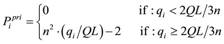
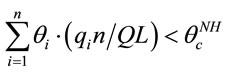
The optimization function (Equation (5-1)) determines the congestion degree in the present node as well as the sending rate in the preceding child nodes. However, the maximum sending rate for the node (equal to the volume of arriving traffic plus the volume of produced traffic) corresponds to the rate determined by the next hop node. Equation 3 is a statement of the mentioned condition. n is the number of upstream neighbors (preceding child nodes), qi the number of packets in the queue related to ith traffic and QL/n is the maximum queue length in ith traffic.
Each node after receiving a set of packets runs the Equation (5-1) function and in case of detecting congestion or an increase in the sending rate of one of the senders, determines the sending rate of the preceding node(s) and provides this rate to the nodes. All q parameters are
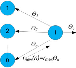
Figure 7. The model used in intermediate nodes.
in the range (0 and 1); 1 meaning that the entire bandwidth can be used and 0 meaning that no data can be sent.
Parameter a determines the importance of congestion in the network. The greater this parameter, the greater the importance of congestion control in the network. For example, if a is set as 1, the factor of qc becomes zero and the value of qc is practically 1. In this case, according to Equation (5-2), the rate of all the senders will be zero. Proposed congestion control mechanism is used only for low priority traffics. Obviously, while the network serves the high priority packets with the highest available resources, it is expected that high priority traffics do not experience congestion. Also, the rate of high priority traffic is much less than low priority.
4. Performance Evaluation of the Proposed Protocol
MATLAB and OPNET [26] are the two software used in investigating the performance of the proposed protocol. The Equation 2 optimization function along with other required functions were run in MATLAB. The simulation phase was carried out using OPNET. The proposed protocol links two softwares. Figure 8 shows the used topology and Table 2 presents parameters used in simulations.
In addition to backpressure methods as factors of evaluating the proposed protocol performance, the REEP [20] protocol was also used. REEP is a data-centric, energy efficient and reliable routing protocol for WSNs. This protocol follows different phases like other data centric protocols for routing which include: Sense event propagation, Information event propagation and Request event propagation. REEP also uses an energy threshold value in order to make the sensor nodes energy-aware. REEP also has five important elements, i.e. sense event, information event, request event, energy threshold value and request priority queue (RPQ).
Data centric Routing protocol REEP uses Flooding to perform the first phase and it has a lower efficiency. HLAF algorithm prevents the wasting of energy by considering new method and provides the possibility of data transmission with different priorities.
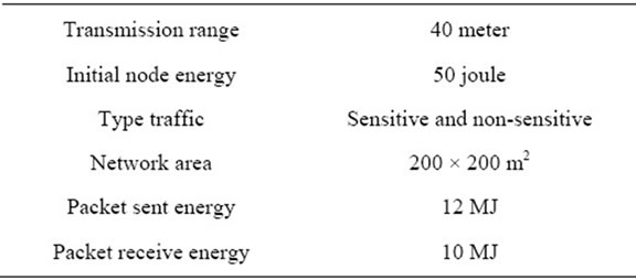
Table 2. Simulation parameters.
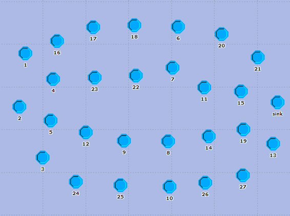
Figure 8. The topology which is used in simulation.
1) HLAF Performance Evaluation In the rest of the paper HLAF and LAF are compared from delay point of view. One of main goals of HLAF is to reduce end to end delay. We will evaluate its performance here. In Figure 9, delay is compared for HLAF and LAF over packet loss rate. Packet loss rate is the rate of packets lost in network links. In this figure, two delay types are presented: the least and the most delay. For determining delay, we consider the node with the longest distance to sink as criterion. With respect to data dissemination mechanism in healthcare Wireless Sensor Networks, in spite of the decrease of number of forwarded redundant packets, totally more than one packet will arrive at destination in both protocols. Each of packets which arrive to criterion node has particular delay. We use the least and the most delay for comparing protocols. As observable in Figure 9 the least delay for HLAF packets is almost half of LAF packets delay. Simulation results are shown for different loss rates. Packets which arrive at destination using shortest path, have the least delay. But loss rate influences on the most delay. When the number of packets decreases, queuing delay decrease too. It can be seen that the least and the most delays for HLAF are less than that of LAF.
In Figure 10 the lifetime is plotted versus packet loss rate. Packet generation rate in sink is considered constant. As can be seen in Figure 10, when packet loss rate increases, network lifetime for both protocols LAF and HLAF increases too. This leads to a decrease in energy consumption of each packet. For example, when packet loss rate is zero, all the packets reach the destination, but when loss rate is more than zero, some of packets are dropped in the path and it causes a decrement in consumed energy.
It is obvious in Figure 10 that network lifetime for HLAF is more than LAF. It means that HLAF is more successful in decreasing number of redundant packets. Whenever sending forwarded packets are prevented, you
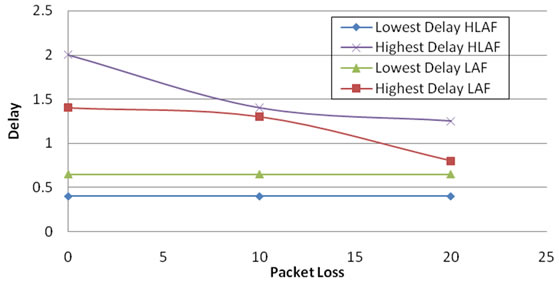
Figure 9. Delay versus loss rate.
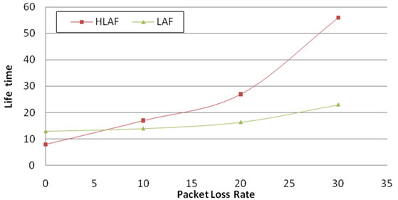
Figure 10. Lifetime versus loss rate.
can save much more energy.
2) Energy Performance Comparison Life time and fairness are two important factors that should be taken into account in evaluating the performance of the proposed protocol. Figure 9 illustrate lifetime of the network. The horizontal axis represents traffic load in kb/s and the vertical axis represents lifetime per time unit. Network lifetime spans from the time the simulation is run until the first node dies.
In Figure 11, the performance of COCM is shown in comparison with REEP from the view of traffic load, which are about 400 packets per time unit. For example, at a traffic load of 200 packets per time unit, COCM increases lifetime in comparison to REEP by about 78 percentages. COCM uses multiple paths to send data. This method ensures fair distribution of traffic at the destination, which increases network life time while the REEP protocol uses one way traffic transmission. We can see in Figure 11 that COCM has a better performance than REEP in terms of network life time.
As we mentioned before, respecting fairness on energy consumption is one of the powerful point of COCM in energy performance. If we can keep better balance in the energy consumption of nodes the lifetime of the network increases under the same conditions. According to Figure 12, fairness parameter is more successful in COCM rather than REEP one. Considered parameter has calculated with Equation (7). Equation (7) calculates the variance of normalized remaining energy of network nodes with initial energy (Emax) to average remained energy (Ave) of total network. In Equation (7), Energyi is node i
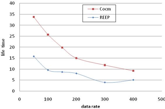
Figure 11. Life time over traffic load.
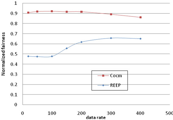
Figure 12. Energy fairness over traffic load.
remaining energy when simulations ends.
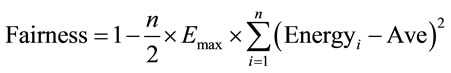 (7)
(7)
As it is clear in Equation (7) the more fairness parameter, the protocol is much success that it means remaining energy of nodes are closer with each other. If fairness parameter is equal one, the network has the best and the most fairness case (all nodes have the same remained energy), however when it is equal zero we have the most unfairness case of energy consumption.
In WSNs, when data converge toward the sink, congestion is more likely to happen at sensors near sink which are likely to receive more data than they can forward. Every near-sink sensor node is a hotspot and so, its resources are more valuable. By providing fairness, network lifetime will be prolonged.
As it is clear in Figure 13 the rate and speed of nodes residual energy for COCM is closer with each other rather than REEP one. There are four nodes with number such as 13, 15, 19 and 21 on sink’s neighborhood. The more increasing life time, the more successful network we have. In order to increase network life time, the traffic near the sink has to distribute among all nodes so that its life time prolongs. In REEP method, all the packets reach to sink by node 15 and other near sink nodes do not participate in traffic pass. So speed of this is less than other nodes and life time of network getting worst. But in proposed method by fair traffic distribution between all nodes, the speed of node energy decreases going to be diminishing so that it causes network longer life time and fairness improvement on energy consumption. In Figure 13, the horizontal axis is time and the vertical axis shows nodes residual energy.
At the end, the total results of Figures 11-13 shows that COCM energy performance is more efficient.
3) Packet Loss Comparison In Figure 14, aggregative packet loss rate over time with initial source rate 200 packets per second has been shown. In this figure COCM protocol in addition to REEP is compared with 25% and 50% backpressures too. Back pressure refers to the backpressure algorithms with 25% and 50% reduction percentages, respectively, in a sensor’s data rate in response to a backpressure message. Horizontal axis is the time and vertical axis shows Aggregative packet loss. The initial source rate in the simulations is 100 packets per second.
As can be seen in Figure 14, due to existing of control packets before the time 10, the possibility of controlling the source rate is a difficult process. Also hop by hop rate
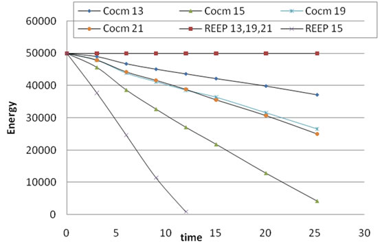
Figure 13. Near-sink nodes energy over time.
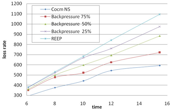
Figure 14. Aggregative packet loss over time.
adjustment from congested node to source node will be accompanied with delay. After time 10 rate adjustment performs efficiently and as a result packet loss rate decreases that can be seen in Figure 14.
We implemented the back pressure algorithms for comparison purposes in our simulations. We have implemented backpressure here instead of proposed congestion control mechanism in COCM. For example, backpressure 25% performs routing process like the COCM, but it uses reduces source rate 25% in response to a congestion notification message. If an upstream node (toward source node) is a data source, it reduces the data generating rate by the same percentage.
In Figure 15 we show packet loss over time. As can be seen in this figure, packet loss rate for COCM is less than other algorithms. The COCM uses efficient congestion control and rate adjustment algorithm and so has less number of packet losses. According to Figure 15 it can be observed that after sensitive COCM, non-sensitive COCM has least number of packet losses. REEP does not have any congestion control procedure and therefore it has the largest number of packet loss.
4) End to End Delay Comparison Another fundamental parameter which is considered in COCM is the end to end delay. Delay is a parameter which is crucially important for the healthcare applications. With regard to the fact that REEP could not have priority for different traffic type, there exists only one priority for it. In Figure 16, end to end delay for sensitive and non-sensitive traffic in COCM and for REEP has been shown.
Due to the fact that it is not possible for REEP to prioritize different types of traffic, it supports only one type. Figure 16 presents the end to end delay in both sensitive and non-sensitive COCM as well as REEP. End to end delay is the time taken for a packet to be transmitted from source to destination. Figure 16 indicates that the end to end delay at the beginning of simulation before time 3 is increasing. This is because of queuing delay of the control packets in the first and second phases. But
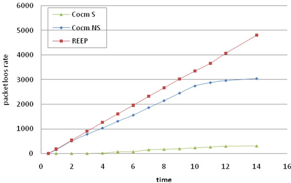
Figure 15. Packet loss over time.
after time 3 all algorithms end to end delay decrease and sensitive traffics end to end is less than both non-sensitive and REEP traffics. Low end to end delay is expected for sensitive traffics considering the scheduler used for them. Simulations show that COCM could achieve its objectives.
Figure 17 shows the mean queue size over time. Mean queue size is a major metric in delay measurement. The more queue size, the more delay. The reason behind the queue size rate being less in COCM is utilizing multipath technique.
5) Bandwidth Performance Bandwidth performance is one of the most important parameters in congestion management methods. As is shown in Figure 18, COCM has much better bandwidth performance compared to REEP. This is mainly because of the large amount of lost packets in REEP. Also CPCM uses different paths to be able to send great amounts of traffic (multipath).
5. Conclusion
In this paper, we presented a congestion management
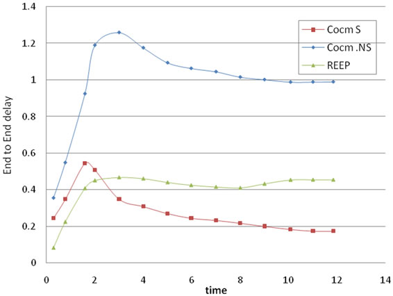
Figure 16. End to end delay over time.
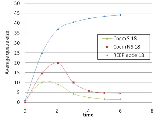
Figure 17. Mean queue size over time.
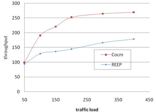
Figure 18. Network throughput over traffic load.
data driven model for use in healthcare wireless sensor networks with stationery patients. This model consists of service differentiation and congestion management (congestion control, congestion avoidance) units. The service differentiation unit supports three kinds of traffics namely, sensitive, non-sensitive, and control packet. The congestion management unit in the first place tries to avoid congestion by a novel multipath routing with different phases: request dissemination, event report, route establishment and data forwarding. In data forwarding phase the high priority data traffic is forwarded through shortest path route to meet the low delay service requirements. The low priority and control traffics are routed through the other routes. In case of congestion occurrence, the proposed congestion control mechanism assigns a new rate for source traffics. The proposed protocol takes into account parameters like end to end delay, energy consumption, lifetime of the network and fairness in energy consumption. Finally, using performed simulations, the performance of COCM has been investigated. Simulation results show that the proposed protocol is more efficient than the backpressure and REEP protocols.
REFERENCES
- I. F. Akyildiz, W. S. Sankarasubramaniam and E. Cayirci, “Wireless Sensor Networks: A Survey,” Computer Networks, Vol. 38, No. 4, 2002. pp. 393-422. doi:10.1016/S1389-1286(01)00302-4
- A. A. Ahmed, H. Shi and Y. Shang, “A Survey on Network Protocols for Wireless Sensor Networks,” International Conference on Information Technology: Research and Education, 11-13 August 2003, pp. 301-305.
- A. Darwish and A. E. Hassanien, “Correction: Darwish, A. and Hassanien, A.E. Wearable and Implantable Wireless Sensor Network Solutions for Healthcare Monitoring,” Sensors, Vol. 12, No. 9, 2012, pp. 12375-12376. doi:10.3390/s120912375
- H. Alemdar and C. Ersoy, “Wireless Sensor Networks for Healthcare: A Survey,” Computer Networks, Vol. 54, No. 15, 2010, pp. 2688-2710. doi:10.1016/j.comnet.2010.05.003
- K. Sha, J. Gehlot and R. Greve, “Multipath Routing Techniques in Wireless Sensor Networks: A Survey,” Wireless Personal Communications, Vol. 70, No. 2, 2013, pp. 807-829. doi:10.1007/s11277-012-0723-2
- A. J. D. Rathnayaka and V. M. Potdar, “Wireless Sensor Network Transport Protocol: A Critical Review,” Journal of Network and Computer Applications, Vol. 36, No. 1, 2013, pp. 134-146. doi:10.1016/j.jnca.2011.10.001
- T. J. Dishongh and M. E. McGrath, “Wireless Sensor Networks for Healthcare Applications,” Artech House, 2010.
- C.-Y. Wan, S. B. Eisenman and A. T. Campbell, “CODA: Congestion Detection and Avoidance in Sensor Networks,” In: Proceedings of the 1st International Conference on Embedded Networked Sensor Systems, ACM, Los Angeles, California, 2003, pp. 266-279. doi:10.1145/958491.958523
- B. Hull, K. Jamieson and H. Balakrishnan, “Mitigating Congestion in Wireless Sensor Networks,” In: Proceedings of the 2nd International Conference on Embedded Networked Sensor Systems, ACM, Baltimore, 2004, pp. 134-147. doi:10.1145/1031495.1031512
- M. H. Yaghmaee and D. Adjeroh, “A New Priority Based Congestion Control Protocol for Wireless Multimedia Sensor Networks,” International Symposium on World of Wireless, Mobile and Multimedia Networks, Newport Beach, 23-26 June 2008, pp. 1-8.
- O. B. Akan and I. F. Akyildiz, “Event-to-Sink Reliable Transport in Wireless Sensor Networks,” IEEE/ACM Transactions on Networking, Vol. 13, No. 5, 2005, pp. 1003-1016. doi:10.1109/TNET.2005.857076
- Y. G. Iyer, S. Gandham and S. Venkatesan, “STCP: A Generic Transport Layer Protocol for Wireless Sensor Networks,” 14th International Conference on Computer Communications and Networks, 2005.
- C. T. Ee and R. Bajcsy, “Congestion Control and Fairness for Many-to-One Routing in Sensor Networks,” In: Proceedings of the 2nd International Conference on Embedded Networked Sensor Systems, ACM, Baltimore, 2004, pp. 148-161.
- C. Wang, et al., “Upstream Congestion Control in Wireless Sensor Networks through Cross-Layer Optimization,” IEEE Journal on Selected Areas in Communications, Vol. 25, No. 4, 2007, pp. 786-795. doi:10.1109/JSAC.2007.070514
- M. M. Monowar, et al., “Congestion Control Protocol for Wireless Sensor Networks Handling Prioritized Heterogeneous Traffic,” In: Proceedings of the 5th Annual International Conference on Mobile and Ubiquitous Systems: Computing, Networking, and Services, ICST Institute for Computer Sciences, Social-Informatics and Telecommunications Engineering, Dublin, 2008, pp. 1-8.
- L. Q. Tao and F. Q. Yu, “ECODA: Enhanced Congestion Detection and Avoidance for Multiple Class of Traffic in Sensor Networks,” IEEE Transactions on Consumer Electronics, Vol. 56, No. 3, 2010, pp.1387-1394. doi:10.1109/TCE.2010.5606274
- A. A. Rezaee, M. Samimi and M. H. Yaghmaee, “Design a New Fuzzy Congestion Controller in Wireless Sensor Networks,” International Journal of Information and Electronics Engineering, Vol. 2, No. 3, 2012, pp. 395-399.
- Y. Xiaoyan, et al., “A Fairness-Aware Congestion Control Scheme in Wireless Sensor Networks,” IEEE Transactions on Vehicular Technology, Vol. 58, No. 9, 2009, pp. 5225-5234. doi:10.1109/TVT.2009.2027022
- F. K. Shaikh, et al., “TRCCIT: Tunable Reliability with Congestion Control for Information Transport in Wireless Sensor Networks,” The 5th Annual ICST Wireless Internet Conference (WICON), Singapore, 1-3 March 2010, pp. 1-9.
- F. Zabin, et al., “REEP: Data-Centric, Energy-Efficient and Reliable Routing Protocol for Wireless Sensor Networks,” IET Communications, Vol. 2, No. 8, 2008, pp. 995-1008. doi:10.1049/iet-com:20070424
- C. Intanagonwiwat, R. Govindan and D. Estrin, “Directed Diffusion: A Scalable and Robust Communication Paradigm for Sensor Networks,” In: Proceedings of the 6th Annual International Conference on Mobile Computing and Networking, ACM, Boston, 2000, pp. 56-67.
- B. Esmailpour, A. Rezaee and J. Abad, “Congestion Avoidance and Energy Efficient Routing Protocol for WSN Healthcare Applications,” In: T.-H. Kim, et al., Eds., Communication and Networking, 2010, Springer, Berlin Heidelberg, pp. 1-10. doi:10.1007/978-3-642-17604-3_1
- H. Sabbineni and K. Chakrabarty, “Location-Aided Flooding: An Energy-Efficient Data Dissemination Protocol for Wireless-Sensor Networks,” IEEE Transactions on Computers, Vol. 54, No. 1, 2005, pp. 36-46. doi:10.1109/TC.2005.8
- H. Wang, C. Liao and Z. Tian, “Effective Adaptive Virtual Queue: A Stabilising Active Queue Management Algorithm for Improving Responsiveness and Robustness,” IET Communications, Vol. 5, No. 1, 2011, pp. 99- 109. doi:10.1049/iet-com.2009.0700
- V. Firoiu and M. Borden, “A Study of Active Queue Management for Congestion Control,” IEEE 19th Annual Joint Conference of the IEEE Computer and Communications Societies, Tel Aviv, 26-30 March 2000, pp. 1435- 1444.
- www.opnet.com