Journal of Water Resource and Protection
Vol.08 No.02(2016), Article ID:63374,8 pages
10.4236/jwarp.2016.82011
Inversion of Seawater Physical Properties Based on Allied Elastic Impedance
Xueqin Liu1, Huaishan Liu1*, Jinqiang Zhu1,2, Jia Wei1
1Key Lab of Submarine Geosciences and Prospecting Techniques, Ministry of Education, Ocean University of China, Qingdao, China
2Geophysical Data Processing & Interpretation Center, China Oilfield Services Limited, Tianjin, China

Copyright © 2016 by authors and Scientific Research Publishing Inc.
This work is licensed under the Creative Commons Attribution International License (CC BY).
http://creativecommons.org/licenses/by/4.0/


Received 17 December 2015; accepted 1 February 2016; published 5 February 2016
ABSTRACT
Inversion of seawater physical parameters (temperature, salinity and density) from seismic data is an important part of Seismic Oceanography, which was raised recent years to study physical oceanography. However present methods have problems that inversion accuracy is not high or inverted parameters are incomprehensive. To overcome these problems, this paper derives Allied Elastic Impedance (AEI), from which we can extract acoustic velocity and density of seawater directly. Furthermore this paper proposes a method to fit temperature and salinity with acoustic velocity and density respectively, breaking through the limitation that temperature and salinity can only be extracted from acoustic velocity. After applying it to model and real data, we find that this method not only solves the problem that ocean density is hard to extract, but also increases accuracy of other parameters, with the temperature and salinity resolution of 0.06˚C and 0.02 psu respectively. All results show that AEI is promising in inversion of seawater physical parameters.
Keywords:
Seismic Oceanography, AEI, Inversion of Ocean Parameters

1. Introduction
As a method to explore geologic structure and hydrocarbon resources by means of wave reflection, multichannel seismic (MCS) has been applied in ocean research for decades. But for a long time, geophysicists are just focusing on the reflections bellow seafloor, while those from seawater are ignored as noises [1] . So reflections from seawater didn’t play a role until Holbrook found the relationship between them and seawater’s thermohaline structure [2] . He believed that multichannel seismic could be used to research physical oceanography, and set up the new subject of seismic oceanography. This new method improves the lateral resolution greatly compared with traditional oceanography measurements.
Early researches of seismic oceanography were mainly focused on describing boundaries of water mass and thermohaline gradient directly by seismic reflections, and some success have been achieved in the study of marine fronts [3] , internal waves [4] , mesoscale eddies [5] and other marine phenomenon. With higher demand for thermohaline structure, precise inversion of seawater’s physical properties seems necessary. In order to analyze ocean structure quantitatively, Wood applied full waveform inversion to synthetic seismogram and real seismic data, and got satisfying results [6] . Afterward Kormann, Bornstein improved full waveform inversion method, increasing the inversion accuracy [7] [8] . Song Hai-Bin also got good profiles with the temperature resolution of 0.16˚C by means of acoustic impedance inversion [9] . However all these methods can’t attain seawater density or fit it with acoustic velocity by empirical formula, which also brings down the accuracy of temperature and salinity. As the main parameter that controls ocean dynamics, seawater density is important to ocean circulation, geostrophic current and other dynamic processes [10] . So this paper presents a new inversion approach, which can resolve acoustic velocity and density simultaneously from a transit parameter allied elastic impedance. On this basis, we fit temperature and salinity with acoustic velocity and density respectively.
2. Allied Elastic Impedance
Zoeppritz equations are used to describe relationship between reflectivity of elastic interface and velocity, density and incident angle of adjacent layers. For liquid interface, it becomes to be [11]
 (1)
(1)
where ,
,  and
and ,
,  are respectively acoustic velocity and density of upper and lower water layer,
  and
and  are angle of incidence and emergence. Variation of ocean parameters is very little, meeting the condition that
 (2)
(2)
where ,
,  are differences of acoustic velocity and density between upper and lower water layer. So we can simplify Equation (1) as
 (3)
(3)
Here we need a function  which has properties similar to acoustic impedance, so that reflectivity can be derived from the formula given for any incidence angle θ
 (4)
(4)
when  changes little, reflectivity can be represented as alternative log derivation
 (5)
(5)
So
 (6)
(6)
 (7)
(7)
Then we substitute  for
for 
 (8)
(8)
Finally we integrate and index Equation (8), setting the integration constant to zero.
 (9)
(9)
We can see the format of  is similar to acoustic impedance and elastic impedance, and we name it allied elastic impedance (AEI) in this paper. It’s not a physical parameter that can be measured directly, but an attribute used to interpret seismic data. Different from acoustic impedance, AEI changes with incidence angle, so it can provide more information. Compared with elastic impedance, AEI doesn’t contain shear wave and have a simpler form, so it is more suitable for inversion.
However, AEI has an undesirable feature that its dimensionality varies with incidence angle θ and provides numerical values that change significantly with θ (Figure 1). For the convenience of comparison, we normalized AEI function by means of v0 which is the average value of acoustic velocity from XCTD [12] .
 (10)
(10)
This is the final form for inversion, and we can see that modifying the AEI function doesn’t affect the value of reflectivity through function (4).
3. Extinction of Seawater Physical Parameters
The inversion of AEI is similar to that of acoustic impedance, which is also performed with the constraint of XCTD. While the input data is angle stack data, the impedance for constraint is calculated by function (10), and the wavelet is extracted from corresponding angle stack data. Low frequency model plays an important role in the process of inversion.
From function (10), we can know that, in order to extract acoustic velocity and density from AEI, at least two allied elastic impedance volumes are needed. So that they can compose simultaneous equations blew.
 (11)
(11)

Figure 1. The variation of elastic impedance (AI) and AEI with incidence angle when density is 1020 kg/m3 and velocity is 1520 m/s.
Here, we replace  with M. The value of M can be got from XCTD and inverted AEI at the corresponding location through function (10). Because M doesn’t change with samples under the same incidence angle, we can take the average value of M from every sample as proper value of M. Then v (acoustic velocity) and ρ (density) can be solved from Equations (11).
Acoustic velocity and density is calculated at every sample separately, leading to the throb of results. Considering that ocean parameters vary very gently, we smooth the inverted profiles by means of cubical smoothing algorithm with five-point approximation, making them closer to the actual situation.
After getting acoustic velocity and density, we can extract temperature and salinity from them. Traditional method looks for the optimum temperature and salinity iteratively by means of empirical velocity equation (Wilson equation) and temperature-salinity relationship from XCTD. However the relationship between them is always complex and nonmonotonic, accurate relationship is hard to get. According to the conclusion that temperature is sensitive to acoustic velocity and salinity is easy to be affected by density [13] , we propose a method to calculate temperature and salinity by acoustic velocity and density respectively, which improves the accuracy of temperature and salinity greatly. Testing several XCTD data, we find that acoustic velocity and temperature have good linear correlation, while relationship between density and salinity is changeable, which can be got by means of artificial neural network.
4. Application on Real Seismic Data
Figure 2 shows two angle stack profiles of seawater from the same cross line of East China Sea. (a) is small angle stack and (b) is large angle stack, from which we can see the variation of amplitude dependent incidence angle. There’s only one simultaneously measured XCTD set on this line at the location of CDP486. Figure 3 shows four curves of velocity, density, temperature and salinity from the XCTD. Combined with the angle stack profiles, we can infer that there’s maybe a halocline at time of 0.15 s. To attain the relationships of acoustic velocity-temperature and density-salinity, we map their crossplots (blue points in Figure 4). According to their distribution shape, we fit the relationships of acoustic velocity-temperature and density-salinity by linear function and artificial neural network respectively (red line in Figure 4). Figure 4 shows the fitting curves have good agreement with the crossplots. So we think of these relationships as the representative relationships in this field and apply them to the whole line.
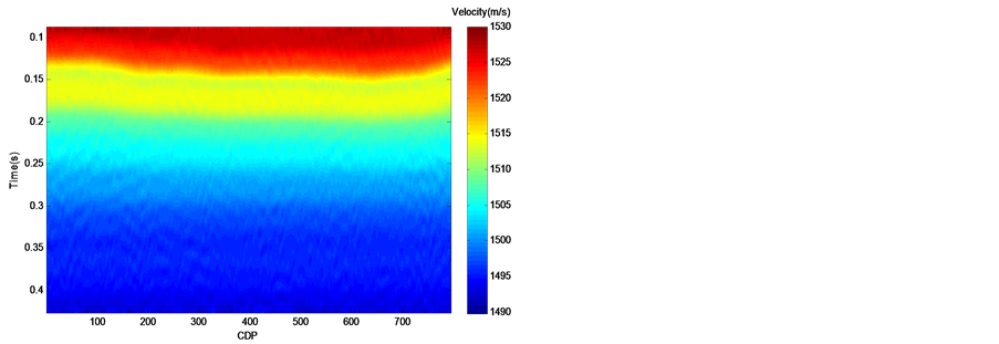
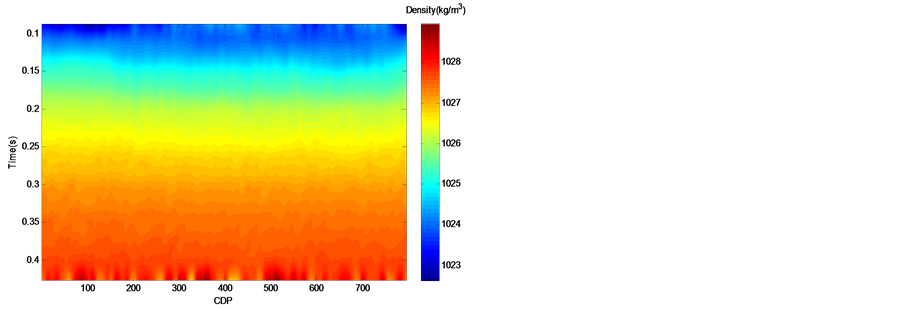
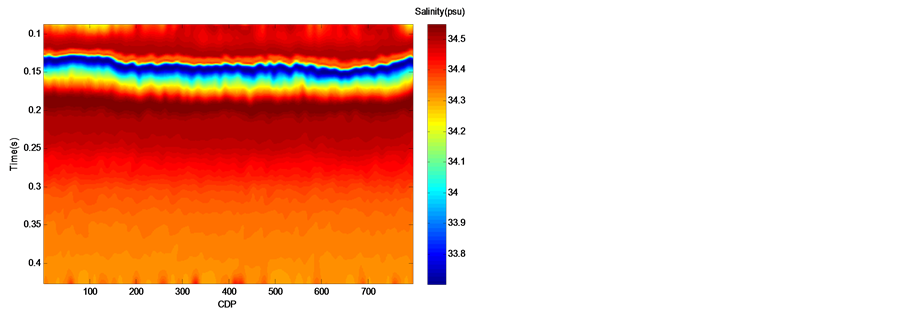
Then we invert AEI from angle stack data with the constraint of XCTD data, resolve acoustic velocity and density from AEI, and compute temperature and salinity by the fitting relationships. Figure 5 shows the final profiles of acoustic velocity, density, temperature and salinity, from which we can see the distribution of each parameter on this profile easily. To analyze the inversion accuracy quantitatively, we extract inverted data at the same location with XCTD and compare these two curves in Figure 6. As can be seen, inverted data and XCTD data get a good agreement. After calculating, the mean errors of acoustic velocity, density, temperature and salinity are 0.05 m/s, 0.03 kg/m3, 0.06˚C and 0.02 psu respectively. Taking their variation ranges into consideration, relative errors of density and salinity are bigger than acoustic velocity and temperature. This is because relative contribution to reflectivity of acoustic velocity and temperature are far greater than density and salinity, and all these results are inverted from reflectivity [14] .
To highlight the variation of temperature and salinity on the profile, we also convert their data maps to contour maps, as shown in Figure 7. Combined with XCTD data, we can draw the conclusion that there’s a halocline at time of 0.15 s nearby.
5. Conclusions
This paper derives AEI from Zoeppritz equations of liquid and resolves acoustic velocity and density from it. Furthermore we propose a method to calculate temperature and salinity. After applying it to real data, we come to following conclusions:
1) Reflections from seawater also have obvious AVO features. AEI derived on this basis can provide more information (incidence angle) compared with acoustic impedance. So we can resolve more parameter (density) from AEI.
2) After attaining precise density, temperature and salinity can be calculated by acoustic velocity and density not only by acoustic velocity, which improves inversion accuracy of all parameters.
3) On the ground that input data are angle stack and incidence angle of water layer just below surface is large,
 (a)
(a)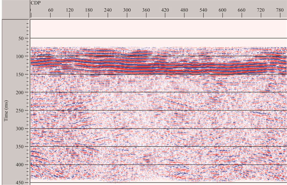 (b)
(b)
Figure 2. Angle stack data of seawater. (a) Small angle stack; (b) Large angle stack.
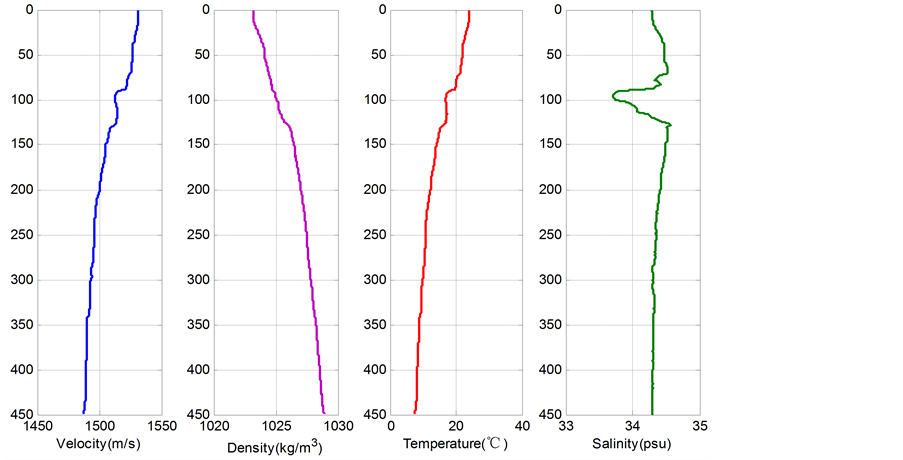
Figure 3. Parameter curves of XCTD.
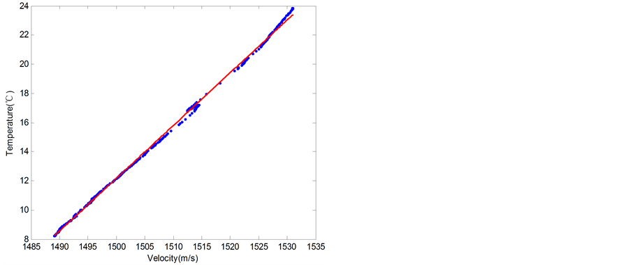
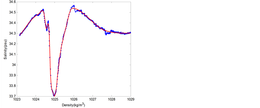
Figure 4. Crossplots and fiting curves of velocity-temperature and density-salinity (blue poits are intersections and red line are fitting curves).
 (a) (b)
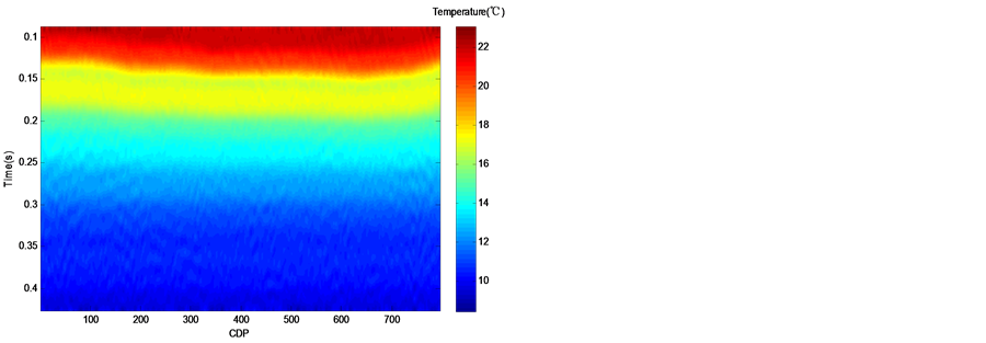
 (c) (d)
Figure 5. Inverted profiles of parameters. (a) Acoustic velocity; (b) Density; (c) Temperature; (d) Salinity.
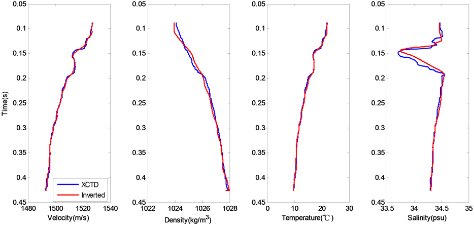
Figure 6. Comparision of curves from XCTD and inverted results at the same position.
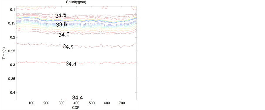
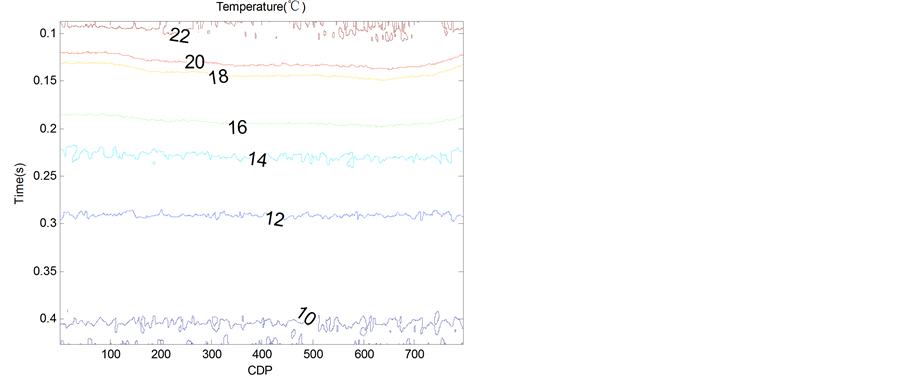
Figure 7. Contour maps of temperature and salinity.
the shallow reflections are easy to be omitted. On the other hand, shallow reflections are mixed with primary waves, so physical parameters of shallow water must be got by other methods.
Acknowledgements
The authors would like to thank the Natural Science Foundation of China (41176077, 41230318), Subject of 863 (2013AA092501), Natural Science Foundation of Shandong (ZR2010DM012), Basic Research Special Foundation of the Third Institute of Oceanography affiliated to the State Oceanic Administration (TIOSOA, 2009004) and the Science Research Project for the South China Sea of Ocean University of China for their financial support to this work.
Cite this paper
HuaishanLiu,XueqinLiu,JinqiangZhu,JiaWei, (2016) Inversion of Seawater Physical Properties Based on Allied Elastic Impedance. Journal of Water Resource and Protection,08,135-142. doi: 10.4236/jwarp.2016.82011
References
- 1. Huang, X.H., Song, H.B., Pinheiro, L.M. and Yang, B. (2011) Ocean Temperature and Salinity Distribution Inverted from Combined Reflection Seismic and XBT Data. Chinese Journal of Geophysics, 54, 307-314.
http://dx.doi.org/10.1002/cjg2.1613 - 2. Holbrook, W.S., Páramo, P., Pearse, S. and Schmitt, R.W. (2003) Thermohaline Fine Structure in an Oceanographic Front from Seismic Reflection Profiling. Science, 301, 821-824.
http://dx.doi.org/10.1126/science.1085116 - 3. Nandi, P., Holbrook, W.S., Pearse, S., et al. (2004) Seismic Reflection Imaging of Water Mass Boundaries in the Norwegian Sea. Geophysical Research Letters, 31, No. 23.
http://dx.doi.org/10.1029/2004GL021325 - 4. Holbrook, W.S. and Fer, I. (2005) Ocean Internal Wave Spectra Inferred from Seismic Reflection Transects. Geophysical Research Letters, 32, No. 15.
http://dx.doi.org/10.1029/2005GL023733 - 5. Biescas, B., Sallarès, V., Pelegrí, J.L., et al. (2008) Imaging Meddy Fine Structure Using Multichannel Seismic Reflection Data. Geophysical Research Letters, 35, No. 11.
http://dx.doi.org/10.1029/2008GL033971 - 6. Wood, W.T., Holbrook, W.S., Sen, M.K., et al. (2008) Full Waveform Inversion of Reflection Seismic Data for Ocean Temperature Profiles. Geophysical Research Letters, 35, No. 4.
http://dx.doi.org/10.1029/2007GL032359 - 7. Kormann, J., Biescas, B., Korta, N., et al. (2011) Application of Acoustic Full Waveform Inversion to Retrieve High-Resolution Temperature and Salinity Profiles from Synthetic Seismic Data. Journal of Geophysical Research: Oceans (1978-2012), 116, C11039.
- 8. Bornstein, G., Biescas, B., Sallarès, V., et al. (2013) Direct Temperature and Salinity Acoustic Full Waveform Inversion. Geophysical Research Letters, 40, 4344-4348.
http://dx.doi.org/10.1002/grl.50844 - 9. Ruddick, B., Song, H., Dong, C., et al. (2009) Water Column Seismic Images as Maps of Temperature Gradient. Oceanography, 22, 192.
http://dx.doi.org/10.5670/oceanog.2009.19 - 10. Gorriz, B.B., Ruddick, B.R. and Sallares, V. (2013) Inversion of Density in the Ocean from Seismic Reflection Data. Proceedings of Meetings on Acoustics, Acoustical Society of America, 19, 005009.
http://dx.doi.org/10.1121/1.4798967 - 11. Zheng, X.D. (1992) Some New Development of AVO Technique. Oil Geophysical Prospecting, 27, 305-317
- 12. Whitcombe, D.N. (2002) Elastic Impedance Normalization. Geophysics, 67, 60-62.
http://dx.doi.org/10.1190/1.1451331 - 13. Sallarès, V., Biescas, B., Buffett, G., et al. (2009) Relative Contribution of Temperature and Salinity to Ocean Acoustic Reflectivity. Geophysical Research Letters, 36.
http://dx.doi.org/10.1029/2009gl040187 - 14. Dong, C.Z., Song, H.B., et al. (2013) Relative Contribution of Seawater Physical Property to Seismic Reflection Coefficient. Chinese Journal of Geophysics, 56, 2123-2132.
NOTES

*Corresponding author.