Journal of Water Resource and Protection
Vol.6 No.8(2014), Article
ID:47010,15
pages
DOI:10.4236/jwarp.2014.68071
Modeling the Hydrological Dynamic of the Breeding Water Bodies in Barkedji’s Zone
Mamadou Bop1, Angelina Amadou2, Ousmane Seidou2, Cheikh Mouhamed Fadel Kébé3, Jacques André Ndione4, Soussou Sambou1, Ibrah Seidou Sanda5
1Laboratoire d’Hydraulique et de Mécanique des Fluides, Département de Physique, Faculté des Sciences et Techniques, Université Cheikh Anta Diop de Dakar, Dakar, Sénégal
2Department of Civil Engineering, University of Ottawa, Ottawa, Canada
3Centre International de Formation et de Recherche en Energie Solaire (CIFRES), Département de Génie Civil, Ecole Supérieure Polytechnique, Université Cheikh Anta Diop, Dakar, Sénégal
4Centre de Suivi Écologique (CSE), Dakar, Sénégal
5Agrhymet Regional Center, Niamey, Niger
Email: mamadou1.bop@ucad.edu.sn, pape4121@yahoo.fr
Copyright © 2014 by authors and Scientific Research Publishing Inc.
This work is licensed under the Creative Commons Attribution International License (CC BY).
http://creativecommons.org/licenses/by/4.0/


Received 14 April 2014; revised 12 May 2014; accepted 8 June 2014
ABSTRACT
Temporary water bodies’ dynamics play an important role in the epidemiological chain-borne diseases such as Rift Valley fever as they are the main breeding habitats for mosquitoes. During the rainy season, hundreds of these temporary water bodies appear and grow in the Ferlo region (Senegal). The purpose of this research is to generate historical and future time series water levels and areas at three temporary ponds located in the environment and health observatory of Barkedji. A simple lumped hydrological model was developed for that purpose. It describes each pond watershed as three interconnected reservoirs: canopy, surface storage and soil storage and uses a linear relation to describe infiltration, percolation and baseflow (out of the soil reservoir). Given the depth of the water table in the region, percolation out of the soil surface is considered lost. Evapotraspiration was calculated using the Penman equation and withdraws water from the canopy and surface water reservoirs. Excess runoff from the soil storage is turned into runoff using a triangular unit hydrograph. The calibration was done using two years of hydrological and climatic data collected during the 2011 and 2012 rainy seasons. The calibration was successful and water level in the two ponds was simulated with a Root Mean Square Error (RMSE) of 11.2 to 15 cm. Because of the short duration of the observation, no validation could be done. Given the excellent agreement of the simulated and observed water levels during the calibration phase, the modeling exercise was considered to be successful. The developed models were used to generate historical time series of pond areas and correlate these to mosquitoes’ infestation in the region. Future time series of pond areas were also generated using downscaled outputs of three regional climate models from the AMMA ENSEMBLES experiment. The generated pond levels and areas are being used to assess the evolution of the disease in the next 40 years.
Keywords:Breeding Areas, Hydrology, Pond Dynamics, Climate Change

1. Introduction
Permanent water bodies are relatively scarce within the Sahel due to the low ratio rainfall to Potential EvapoTranspiration (PET). Nonetheless, a large number of temporary ponds collect rainwater throughout the wet season which is often used by villagers for breeding and domestic purposes. Thus, the socio-economic impact is important as they relieve the population from the continual quest for water provided they are well repleted. Unfortunately, these short-term basins remain a vital link in the epidemiological chain of species such as Rift Valley Fever (RVF) [1] . The RVF is a zoonotic disease caused by an arbovirus of the family Bunyaviridae, genus Phlebovirus, responsible for modest ruminants necrotizing hepatitis, abortion, and perinatal mortality in humans. The RFV can trigger pathologies ranging from influenza-like illness to extreme varieties of haemorrhagic icterus syndrome, encephalitis and chorioretinitis. Discovered for the first time on the Rift Valley in Kenya in 1931, the RVF quickly spread in Africa with few cases detected in Yemen and Asia. Furthermore, Senegal has experienced an outbreak of RVF in 1978 [2] -[4] . The RVF is now a growing health problem in West Africa [5] . In Senegal, morbidity associated with RVF epidemics is on the rise [6] . Additionally, an increase in morbidity associated with RVF in Senegal was acknowledged by [6] . Consequently, The RVF has become a growing health problem in West Africa [7] . Several studies revealed the relationship of the disease associated with rainfall and pond dynamics in the Barkedji region in Senegal and multiples indices were developed to link the disease incidence with precipitation and vegetation indexes extracted from satellite images [8] -[10] . [11] designed an agent model to simulate the transmission and spread of the disease around Barkedji. [12] showed that mosquito abundance pertains to different filling stages of ponds thus to analyze the particular epidemiology associated with RVF. [3] [13] developed a mathematical model of the dynamics of populations of Aedes and Culex as a function of the variations of environmental condition of the breeding habitats (water levels and pond areas), suggesting that time series of pond characteristics are important explanatory factors for the prevalence of the disease. A first attempt to model ponds dynamics in the Ferlo region was done by [12] , but the lack of data about pond bathymetry forced them to assume simplified relations for the stage-area relationships of the ponds.
The purpose of this paper is to develop a simple hydrological model of pond dynamics that can be used to generate time series of water levels and surface areas at three ponds located in the Barkedji region in Senegal (Figure 1). Once the model is calibrated for a given pond, historical water levels and pond areas can be rebuilt using historical information at the site or at a neighbor station; future water levels and pond areas can be generated using downscaled regional climate models outputs. The generated time series can be used in combination with the previously mentioned RVF risk assessment methodologies to generate long time series of RVF risk indices which can be used by Senegalese decision makers to understand how the prevalence of the disease may evolve in the coming decades. The present paper is organized as follow: the study area and the characteristics of the three ponds are presented in Section 2. The climatic data sets used for model calibration and hydrological time series generation for past and future periods are presented in Section 3. The hydrologic model architecture is described in Section 4, while the methodology used for calibration and generation of hydrologic time series is explained in Section 5. Results discussion is provided in Section 6 followed by conclusion in Section 7.
2. Study Area
The Ferlo region is located in Northern Senegal (Figure 1) and lies between 300 mm and 500 mm isohyets. Its climate is characterized by two seasons: a dry season spanning over 8 to 9 months and a rainy season lasting 3 - 4 months with an average annual rainfall of 396.3 mm during the 1961-2007 periods [14] [15] . The terrain is flat with an average elevation of 25 m and consists of lateritic soil, uncovered sandy hills stabilized by vegetation [15] -[17] .
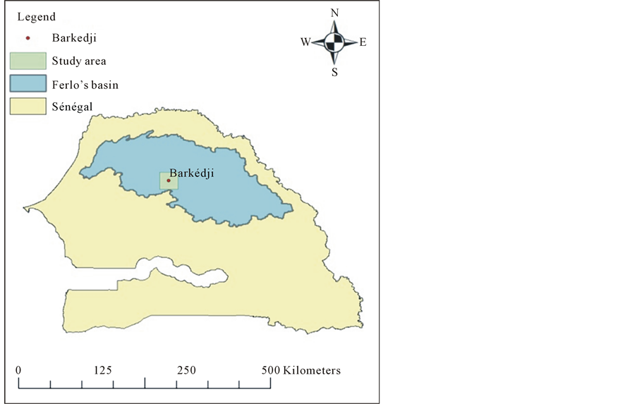
Figure 1. Map of the study area.
The Ferlo is a fossil valley in the Senegal River watershed. It consists of a series of ponds located at the old alluvial channels of the river (the Bounoun). These temporary ponds fill up rather quickly throughout and immediately following the rainy season with draining episodes which may last from few weeks to few months [18] . Barkedji is a Senegalese town (15.277˚N and 14.866˚W) located in the Ferlo valley. The present article focus on three ponds located close to Barkedji. The characteristics of the three ponds are listed in Table1
3. Past, Present and Future Climatic Data
3.1. The QWeCI Data Collection Program
The area of Barkédji (15.277˚N and 14.866˚W) has been identified as Environment and health observatory by the QWeCI (Quantifying Weather and Climate Impact on health on the developing countries) program, and a monitoring network has been installed in 2010 to collect hydrologic and climatic data by the QWeCI program. The climatic and meteorological network consists of 10 (ten) tipping bucket rain gages providing rainfall and temperature data at a 5-minute time step and 2 (two) weather stations providing rainfall, temperature, speed and direction’s wind, solar radiation, humidity, potential evaporation and pressure at a 1hour time step. That rain gauges and weather stations are installed near the selected sentinel ponds and collect data during 2010-2011 and 2011-2012 rainy seasons, thereby 84 (eighty four) rain events are recorded. The hydrometrical equipment consists of OTT staff gages installed inside the ponds and providing the water level at a 1 day time step. The location and characteristics of the measurement devices are listed on Table1 The collected data (rainfall, temperature, potential evaporation and water level) during the 2010-2011 and 2011-2012 rainy seasons (June to September) was used to calibrate model on the (3) three ponds.
3.2. Historical Data at the Linguère Station
The Linguère Station (longitude = −15.21˚; latitude = 15.38˚) is the closest climatic station with available historical measurements of precipitations and temperature. The 1980-2007 precipitation and temperature of the station were acquired and used to force the hydrological models. Relative humidity, wind speed and solar radiations were extracted from NCEP global data sets.

Table 1. Characteristics of the hydro-climatic equipment.
3.3. Available Climate Models Outputs
AMMA-ENSEMBLES is an international collaborative model intercomparison experiment [19] that resulted in a set of regional climate model (RCM) simulations covering most of the African continent at a resolution of 50 km. The RCMs were driven by either the ERA-INTERIM reanalysis, or by global climate models outputs simulated under the SRES A1B emission scenarios. The data sets are available free of charge in the experiments online database (http://ensemblesrt3.dmi.dk/). Nine different RCM/GCM combinations (listed in Table 2) were selected from the AMMA-ENSEMBLE database. All RCM were run on the 1950-2050 period under the SRES A1B scenarios. The simulated precipitation, minimum and maximum temperature time series of the nine GCM/ RCMs combinations were extracted for the Linguére’s station and used in the analysis. The use of an ensemble of different climate simulations allow an evaluation of the uncertainties in individual projections resulting from the RCM/GCM models combination.
3.4. Downscaling of the RCM Outputs
The objective of the procedures described in this section is to apply a transformation to the outputs of a climate model so that the magnitude and distribution of the transformed variable become closer to those of observations at a given point. The gridded precipitation (PCP), wind speed (WND), maximum (MAX) and minimum (MIN) temperature data sets simulated over West Africa by the nine RCM described in the previous section were downloaded from the AMMA-ENSEMBLES data portal. The time-series of each variable were extracted for the Linguère station. A nearest neighbour approach (described later in the section) was used to estimate the two remaining variables (relative humidity and solar radiation). Both the quantile-quantile transformation and nearestneighbour search were done on a monthly basis.
3.4.1. Quantile-Quantile Transformation of RCM Precipitation, Wind Speed and Temperatures
The quantile-quantile transformation, also called quantile-mapping or quantile matching, aims to make the statistical distribution of a given climate variable as close as possible to the statistical distribution of the observed
Table 2 . Characteristics of the three ponds.
variable on the historical period. The transformation for a given month and a given variable is performed as follow:
1) The historical data is split in a calibration period and a validation period. The calibration and validation were set to have the same length. The calibration period is obtained by picking every other year in the observation starting from the first year on the observations. The remaining data set is used for validation. The daily time series of the month are extracted for the associated periods from both observations and RCM simulations.
2) An empirical cumulative distribution function FOBS is developed using the observations on the calibration period; another cumulative distribution function is FRCM is developed using the RCM outputs on the calibration period.
3) Corrected RCM simulations are generated on the validation period and future periods using the following transformation:  where XRCM is the variable extracted from raw RCM simulations and XCORR is the corrected variable.
4) For all variables except precipitation, empirical probability distributions functions (PDF) of the observed, RCM-simulated and corrected variable are plotted and visually compared on both the calibration and validation periods. The probability mass function (PMF) of precipitation occurence (defined as intensity >1 mm/day) as well as the PDF of precipitation intensity on rainy days are generated. If the PDF (or PMF) of corrected variable is closer to the PDF of the observations than the PDF (or PMF) of the non-corrected variable, the quantilequantile transformation is applied to future RCM simulations of that particular variable.
3.4.2. Nearest Neighbour Search for Relative Humidity and Wind Speed
Future values of relative humidity (HMD) and solar radiations (SLR) were generated using a nearest neighbour approach: for each day df in the future period, a day dh is selected in the hitorical period so that it is from the same month as df and the absolute difference between the closest average temperature of df and the average temperature of dh is minimum. The measured solar radiation and relative humidity of dh is assigned to df.
4. The Hydrological Model
Given the small size of the ponds, a simple four-storage conceptual model was developed (Figure 2). Storages in the following components were explicitly simulated:
Canopy storage : represents the amount of precipitation intercepted by vegetation and returned to the atmosphere by evaporation. It is supposed to have a maximum value
  above which the excess water reaches the ground. The canopy storage at time t + 1 is calculated by adding precipitation and removing evapotranspiration of time t. Deficits are transferred to surface storage as remaining evaporative demand (
 ).
).
Surface storage : represents the amount of water which is trapped in depressions on the watershed surface. It is supposed to have a maximum value
  above which the excess water reaches the pond. The rate of which excess water reaches the storm is determined using a triangular unit hydrograph of base tb and time to peak
 . Water can leave surface storage by evaporation and infiltration. The surface storage at time t + 1 is calculated by adding water spilling from the canopy storage and removing infiltration and evaporative demand
  if any. If a deficit occurs immediately after
  to soil storage as remaining evaporative demand (
 ).
).
Soil storage : represents the amount of water which in the soil profile. It is supposed to have a maximum value
  above which infiltration is precluded. Infiltration rate is equal to
  if
if , where Ci is the infiltration coefficient. A fraction
 ![]() (called the tension storage ratio) of the soil storage represents the tension storage and can only leave the soil profile by revaporation. The remaining part
(called the tension storage ratio) of the soil storage represents the tension storage and can only leave the soil profile by revaporation. The remaining part  represents the free-moving part of the soil water and can leave the soil profile by revaporation,
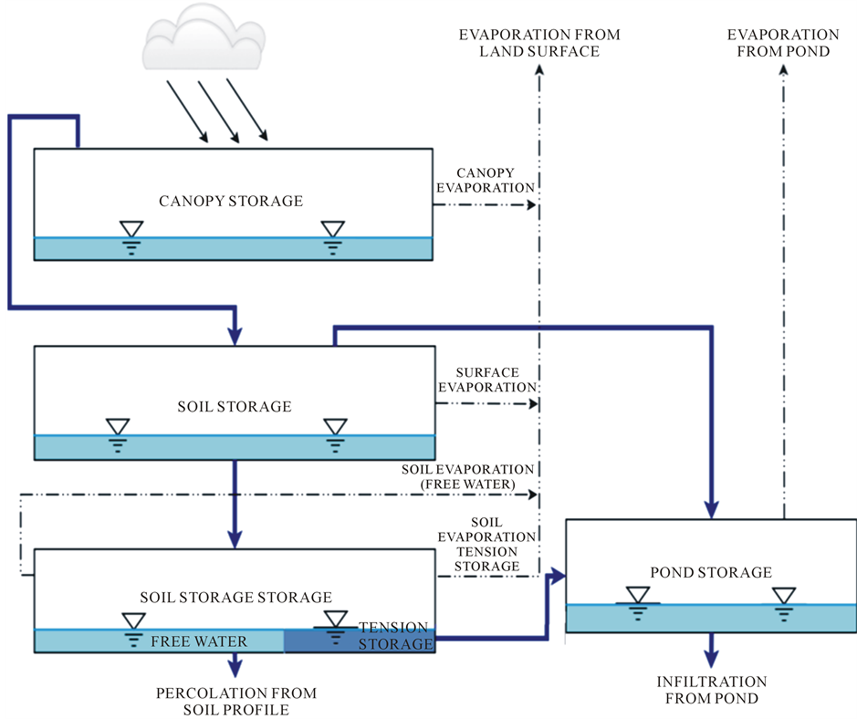
Figure 2. Conceptual representation of the watershed.
interflow (towards the pond) or percolation. Subsurface flow to the pond  is calculated as
 if free-moving water is available. Percolation flow
  is calculated as
  if free-moving water is available.
  and
and  are the soil percolation and the subsurface flow coefficients. Finally, revaporation is calculated as
  where
where  is the soil revaporation coefficient. Subsurface flow and percolation can remove only free moving water, while revaporation tries to remove free moving water first, after tension storage water when no free moving water is available.
Pond Storage : It represents water storage inside the pond and is calculated by mass balance using inflow from the watershed at time, evaporation and infiltration from the pond. Evaporation from the pond is calculated as
  where
where  is the pond area (calculated using the storage and the area-volume relationship of the pond) and
  the pan coefficient. Infiltration is calculated as
  where
where  is the infiltration coefficient.
5. Calibration of the Hydrologic Models and Hydrological Time Series Generation
5.1. Model Calibration
Given that only two years of data were available, only a calibration step was performed. The three hydrological models of the three ponds were calibrated using a combination of trial and errors, and automatic calibration using Excel solver. The objective of the process is to minimize the root mean square error between measured and observed levels.
5.2. Regeneration of Historical and Future Levels and Areas
The 1980-2007 observation data of the Linguère station were used to force the three hydrological models. The downscaled outputs of the nine RCM/GCMs were downscaled at the Linguere station using the methodology described in Section 3.4 and used to force the model.
6. Results and Discussion
6.1. Model Calibration
A set of optimal parameters (listed in Table 3) were found for each of the three ponds by minimising the sum of square error between observed and simulated levels using Excel Solver. The root mean square error (resp. the Nash Suttcliffe coefficient) was 0.15 m (resp 0.80) for Kangueledji, 0.19 m (resp 0.78) for Ngao and 0.112 m (resp. 0.99) for Niakha. The root mean squarre error is respectively 9%, 24% and 8.5% of maximum water levels at kangueledji, Ngao and Niakha. These Nash coefficients are in the same order of magnitude as those obtained in [12] for other ponds in the Ferlo region. Observed and simulated pond levels are presented on Figure 3.
6.2. Downscaling Results
The results of the downscaling experiment at Linguère for the aforementioned six RCMs and six climate variables are presented in Table 4 for all nine RCMs, for three periods( before 2007, 2013-2025 and 2026-2050). Given that the RCM outputs start at different dates, the lengths of the data sets for the historical period (before 2007) are not identical. Three out of nine RCMs suggest an increase in precipitation (up to +47%) in the 2013- 2025 period compared to the historical period, while six RCMs point to a decrease (up to −19.5%) for the same period. Eight out of nine RCMs suggest a decrease in mean precipitation between 2026 and 2050 (up to −24%). An increase in precipitation of +36.7% is projected by CHMIALADIN. The projected increase in maximum temperature between 2013-2025 period and historical period ranged from +0.3˚C (CHMIALADIN) to +0.8˚C (DMI-HIRHAM5, INMRCA3 and MPI-M-REMO). It varies from +1˚C to (CHMIALADIN) to +2.6˚C (INMRCA3) for the 2026-2050 period. The projected increase in minimum daily temperature between 2013- 2025 period and historical period ranged from +0.8˚C (CHMIALADIN) to +1.1˚C (MPI-M-REMO) with a variation of +1.3˚C (GKSS-ECHAM5) to +2.4˚C (INMRCA3) for the 2026-2050 period. All models except REGCM3 predict a slight decrease (equal or less than 1.4%) of relative humidity during the 2026-2050 period. All RCMs point to a decrease in the 0.6% - 2% for relative humidity during the 2026-2050 period. All models suggest wind speed will be lower in both future periods, while solar radiations will undergo very low variations ranging from −0.2% to +0.5% in the 2013-2025 period. All models project a slight increase of up to +0.4% in solar radiation during the 2026-2050 period.
Table 3. Acronyms, origin and data availability for the nine GCM/RCM combinations used.
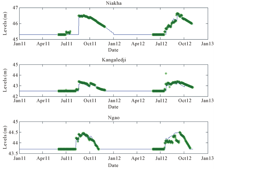
Figure 3. Observed and simulated pond levels.
Table 4. Optimal hydrological model parameters.
6.3. Historical and Future Water Levels and Areas
Figures 4-6 represent the reconstituted 1981-2007 water levels for Kangueledji, Niakha and Ngao ponds. On each figure, pond levels are on the lower part of the graph and should be read on the left y-axis. Pond areas are upside-down on the upper part of the graph and should be read on the right y-axis. The graph shows a lot of inter-annual variability in maximum water levels and areas. Niakha and Ngao display their highest water level in
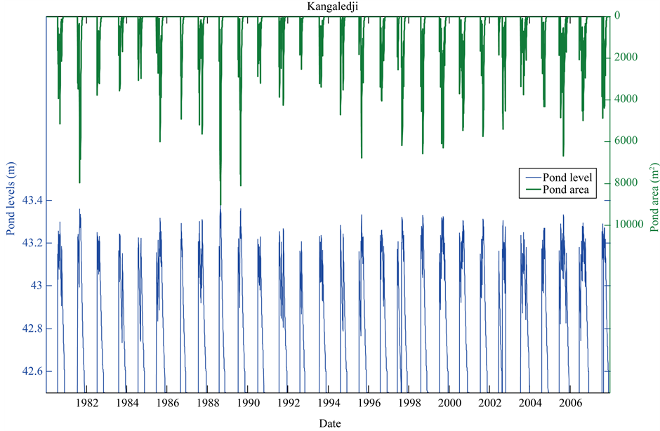
Figure 4. Reconstituted pond levels and areas at Kangeledji.
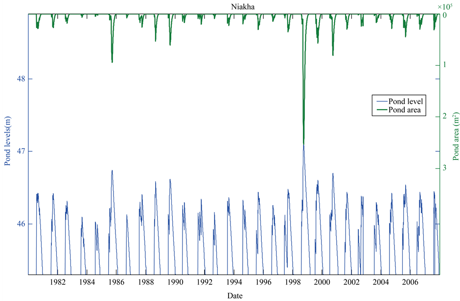
Figure 5. Reconstituted pond levels and areas at Niakha.
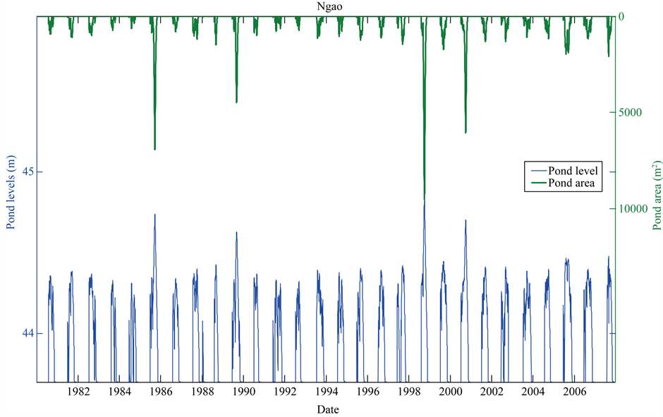
Figure 6. Reconstituted pond levels and areas at Ngao.
historical level at all ponds in 1998 while Kangueledji’s highest water level occurs in 1988. The lowest maximum water level at Kangueledji occurs in 1992 (Table 5) whereas Niaka and Ngao display a lowest maximum water level in 1984. The ratio of the maximum pond area in wet years to the maximum pond area in dry years is 3.6 at Kangueledji, but increases to 15.8 at Ngao and 52.7 at Niakha. As a result, the latter ponds are extremely sensitive to amount of precipitation. Dryer environment in the long term will spur RVF extinction, while a wetter environment may convey a significant increase in RVF.
6.4. Future Water Levels and Areas
Given that water levels are linked to pond areas by the level-volume relationship, only the water levels statistics were extracted and analyzed. Box-plots of simulated daily water levels at Kangueledji, Niakha and Ngao for the June-October period are presented in Figures 7-9 respectively. On each figure, the box-plots are presented for historical (before 2007), 2013-2025 and 2026-2050 periods. The median water levels as well as the upper and lower quartiles are displayed in Table5 The upper panel in each figure shows a variation of the median and the inter-quartile range according to the climate model. This may however be due to the time span of the data sets before 2007 which is different. Some of the RCM outputs (e.g. CHMIALADIN) do not intersect the time span of the observations. Consequently, it was not possible to select a common period to compare the statistics of the water levels simulated with the observations to the statistics of the water levels simulated with the RCMs under the current climate. The middle and lower panels in each figure were generated with data sets of the same length. Three RCM models (CHMIALADIN, KNMI-RACMO and METNOHIRHAM) suggest the median water level as well as the upper quartile will be higher than its historical value at all ponds during the 2013-2025 period, while all the RCMs point to a decrease of the same variables water level for the same period (Figures 7-9, middle panel). Regarding the 2026-2050 period, all models except CHMIALADIN suggest that the median water level, the upper and lower quartile will be lower than during the historical period (Figures 7-9, lower panel).
6.5. Discussion
The study suggests that the ponds are going to be lower in the future than their historical values. Therefore, the
Table 5 . Projected changes in precipitation, temperatures, wind, relative humidity and wind speed at the Lingered station for each of the nine GCM/RCM combinations.
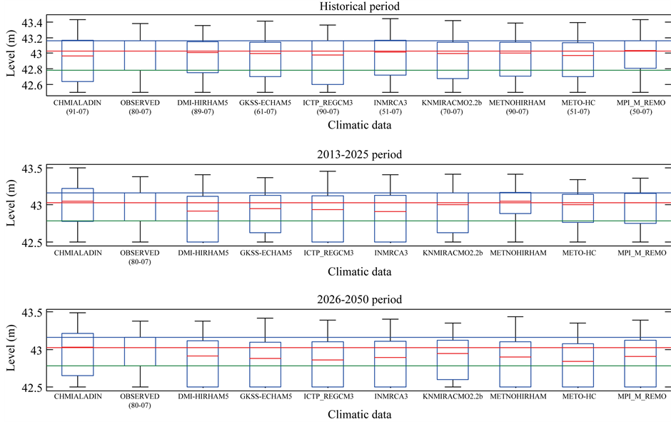
Figure 7. Projected pond levels and areas at Kangeledji (dotted lines: historical upper and lower quartiles; the dashed line: historical median).
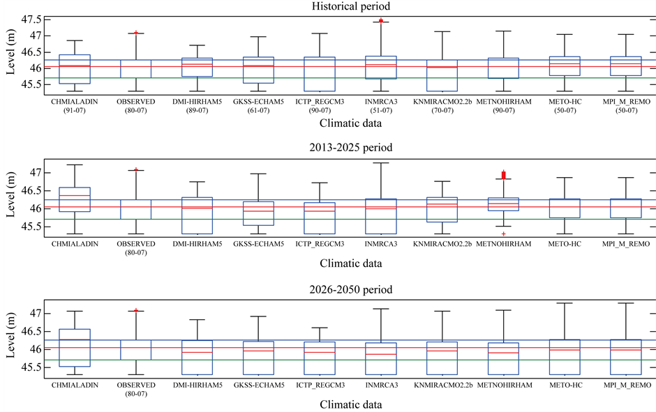
Figure 8. Projected pond levels and areas at Niakha (dotted lines: historical upper and lower quartiles; the dashed line: historical median).
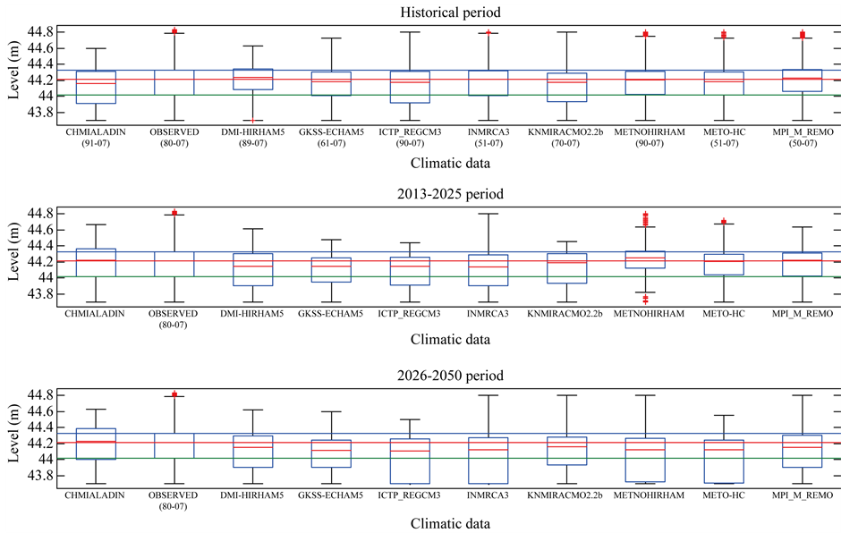
Figure 9. Projected pond levels and areas at Ngao (dotted lines: historical upper and lower quartiles; the dashed line: historical median).
problem the populations will face in the future will probably be the use of the water for breeding and domestic use, as well as a possible deterioration of the quality of the water given the reduction of pond volume. Does this mean a lower prevalence of the RVF in the region? The answer is not easy to give before a model linking the prevalence of the RVF to various parameters among which rainfall regime, pond perimeters and surface. It has been reported that mosquitoes’ abundance and species seem to be a function of vegetation cover and turbidity within ponds [5] [7] [9] . Lower pond levels may translate into higher turbidity and more vegetation as more surface of the pond becomes shallow enough for aquatic vegetation to grow. [13] have proposed a model that allows the calculation of the local abundance of mosquito vectors as a function of the variations the pond levels. The model was not calibrated because of the absence of historical limnigraphic data and mosquitoes abundance. [20] combined a hydrologic pond model with mosquitoe population model to simulate mosquito abundance. Some of the parameters of their model were estimated with literature data and expert knowledge. In the last ten years, several institutions in Africa have been conducting regular entomological studies and fairly long time series of mosquitoes abundance are available, but hydrologic data pertaining to pond dynamic is still missing. Studies such as the one presented in this paper fill the gap by providing such information, and therefore allows the calibration and validation mosquitoes prevalence models. Once these models are calibrated, the downscaled climate data and the projected pond characteristics will provide an insight on the prevalence of the disease in the future. The results presented in this paper are a first step in that direction.
7. Conclusion
A simple three reservoirs hydrological model has been used to simulate the water level dynamics of three temporary ponds in the Ferlo region in Senegal. The models were used to generate historical and future water levels under SRES scenario A1B using the outputs of nine RCMs from the AMMA-ENSEMBLES experiment. The vast majority of the models (eight out of nine) suggested the median and the upper quartiles or the water levels will be lower in the 2026-2050 period. The dryer ponds do not necessarily mean a lower prevalence of the Rift Valley Fever as droughts may result in shallower ponds with more aquatic vegetation and more turbidity, factors which are known to affect mosquitoes’ abundance. The only way to have an accurate idea of the future prevalence is to use the generated time series of pond characteristics with collected mosquitoes’ abundance data to calibrate and validate mosquito prevalence models.
Acknowledgements
This study was funded by the EU project QWeCI (Quantifying Weather and Climate Impacts on health in developing countries; funded by the European Commission’s Seventh Framework Research Programme under the grant agreement 243964).
References
- Molez, J.F., Diop, A., Gaye, O., Lemasson, J.J. and Fontenille, D. (2006) Malaria Morbidity in Barkedji, Village of Ferlo, in Senegal Sahelian Area. Bulletin de la Societe de Pathologie Exotique, 99,187-190.
- Thiongane, Y., Thonnon, J., Zeller, H., Lo, M.M., Faty, A., Diagne, F., Gonzalez, J., Akakpo, J.A., Fontenille, D. and Digoutte, J.P. (1998) Donnees Recentes de l’Epidemiologie de la Fievre de la Vallee du Rift (FVR) au Senegal. Bulletin de la Societe Medicale d’Afrique Noire de Langue Francaise, 1-6.
- Bicout, D.J. and Sabatier, P. (2003) Mapping Rift Valley Fever Vectors and Prevalence Using Rainfall Variations. Vector Borne and Zoonotic Diseases, 4, 33-42. http://dx.doi.org/10.1089/153036604773082979
- Lancelot, R., Gonzalez, J.P., Le Guenno, B., Diallo, B.C., Gandega, Y. and et Guillaud, M. (1989) Epidemiologie Descriptive de la Fievre de la Vallee du Rift chez les Petits Ruminants au sud de la Mauritanie Apres L’hivernage 1988. Revue d’Elevage et de Medecine Veterinaire des Pays Tropicaux, 42, 485-491.
- Chevalier, V., Lancelot, R., Thiongane, Y., Sall, B. and Mondet, B. (2005) Incidence of Rift Valley Fever in Small Ruminants in the Ferlo Pastoral System (Senegal) during the 2003 Rainy Season. Emerging Infectious Diseases, 11, 1693-1700. http://dx.doi.org/10.3201/eid1111.050193
- Ndione, J.A., Besancenot, J.P., Lacaux, J.P. and et Sabatier, P. (2003) Environnement et Epidemiologie de la Fievre de la Vallee du Rift (FVR) dans le Bassin Inferieur du Fleuve Senegal. Environnement, Risques et Sante, 2, 176-182.
- Chevalier, V., Mondet, B., Diaite, A., Lancelot, R., Fall, A.-G. and Poncon, N. (2004) Exposure of Sheep to Mosquito Bites: Possible Consequences for Transmission Risk of Rift Valley Fever in Senegal. Medical and Veterinary Entomology, 18, 247-255. http://dx.doi.org/10.1111/j.0269-283X.2004.00511.x
- Bicout, D.J., Porphyre, T.J.-A. and Sabatier, P. (2004) Modelling Abondance of Aedes and Culex ssp in Rain Fed Pnds in Barkedji, Senegal. Proceedings of the 10th International Symposium on Veterinary Epidemiology and Economic. www.sciquest.org.nz
- Lacaux, J.P., Tourre, Y.M., Vignolles, C., Ndione, J.A. and Lafaye, M. (2007) Classification of Ponds from High-Spatial Resolution Remote Sensing: Application to Rift Valley Fever Epidemics in Senegal. Remote Sensing of Environment, 106, 66-74. www.elsevier.com/locate/rsehttp://dx.doi.org/10.1016/j.rse.2006.07.012
- Ndione, J.A., Lacaux, J.P., Toure, Y., Vignolles, C., Fontanaz, D. and Lafaye, M. (2009) Mares Temporaires et Risques Sanitaires au Ferlo: Contribution de la Teledetection pour L’etude de la Fievre de la Vallee du Rift Entre Aout 2003 et Janvier 2004. Secheresse, 20, 153-160.
- Cisse, A., Bah, A., Drogoul, A., Cisse, A.T., Ndione, J.A., Kebe, C.M.F. and Taillandier, P. (2012) Un Modele à Base Dagents sur la Transmission et la Diffusion de la Fievre de la Vallee du Rift à Barkedji (Ferlo, Senegal). Studia Informatica Universalis, 77-97.
- Soti, V., Puech, C., Lo Seen, D., Bertran, A., Vignolles, C., Mondet, B., Dessay, N., et al. (2010) Thepotential for Remote Sensing and Hydrologic Modelling to Assess the Spatio-Temporal Dynamics of Ponds in the Ferlo Region (Senegal). Hydrology and Earth System Sciences, 14, 1449-1464.
- Porphyre, T., Bicout, D.J. and Sabatier, P. (2005) Modelling the Abundance of Mosquito Vectors versus Flooding Dynamics. Ecological Modelling, 183, 173-181. http://dx.doi.org/10.1016/j.ecolmodel.2004.06.044
- Bop, M. (2008) Impact du Fonctionnement Hydrologique d’un Bassin Endoreique sur la Dynamique des Moustiques: Cas des mares de Barkedji. Memoire de DEA, Universite Cheikh Anta Diop.
- FAO (1999) Schema Directeur de la Zone Ecogeographique Sylvopastorale (Ferlo):Appui au Programme National de la Foresterie Rurale du Senegal,. 14-21.
- Bingham Le Houerou, H.N. (1988) Relationship between the Variability of Primary Production and the Variability of Annual Precipitation in World Arid Lands. Journal of Arid Environments, 1, 1-18.
- Pin-Diop, R., Toure, I., Lancelot, R., Ndiaye, M. and Chavernac, D. (2007) Remote Sensing and Geographic Information Systems to Predict the Density of Ruminants, Hosts of Rift Valley Fever Virus in the Sahel. Veterinaria Italiana Series, 42, 675-686.
- Martin-Rosales, W. and Leduc, C. (2003) Variability of the Dynamics of Temporary Pools in Semi-Arid Endoreic System (Southwestern Niger). Hydrology of Mediterranean and Semi-Arid Regions, 174-178.
- Paeth, H. (2011) Postprocessing of Simulated Precipitation for Impact Research in West Africa. Part I: Model Output Statistics for Monthly Data. Climate Dynamics, 36, 1321-1336. http://dx.doi.org/10.1007/s00382-010-0760-z
- Soti, V., Puech, C., Lo Seen, D., Bertran, A., Vignolles, C., Mondet, B., Dessay, N., et al. (2012) Comuning Hydrology and Mosquitoes Populations Models to Identify the Drivers of Rift Valley Fever Emergence in Semi-Arid Regions of West Africa. PLOS Neglected Tropical Diseases, 6, e1795.