Journal of Water Resource and Protection
Vol. 1 No. 4 (2009) , Article ID: 756 , 12 pages DOI:10.4236/jwarp.2009.14029
Modelling the Financial Value of the Maroochy River to Property Values: An Application of Neural Networks
1CSIRO Sustainable Ecosystems 306 Carmody Road, St. Lucia Queensland, 4067, Australia
2CSIRO Sustainable Ecosystems PO Box 56, Highett, VIC, 3190, Australia
E-mail: {Andrew.higgins, Leonie.pearson, Luis.laredo}@csiro.au
Received June 17, 2009; revised July 15, 2009; accepted September 6, 2009
Keywords: Natural Asset, Financial Value, Neural Network
ABSTRACT
The Maroochy River, which is located on east coast of Australia, provides a variety of uses and values to the community. Changes in structure, function and management of the river will influence the value that the community derives from it. Therefore, critical to the river’s continued management is the development of policy relevant tools based on the community’s value of the river. This paper focuses on estimating the financial value the local residents derive from living close to the river through investigation of changes in residential property values due to attributes of the Maroochy River. It is a complex analysis since there are several confounding geographical and property variables. Given a large and complete dataset of 28,000 properties for the Maroochy region, Artificial Neural Networks (ANN) was applied to estimate the economic value of the properties. This ANN was then able to simulate scenarios for property values with respect to changes in environmental features. It showed the Maroochy River contributed AU$900,000,000 to the unimproved capital value of the whole region, a value that could not be estimated previously, and much higher than anticipated. Calculating potential annual payments to the Shire Council through land tax analysis from these property values, provides the council with means to justify expenditure to maintain a standard of water quality and ecosystem health.
1. Introduction
Estimating the economic value of natural assets, such as river systems, has become a topic of considerable interest by local governments in recent years. It provides a means for justifying different levels of expenditure for improving ecosystem function and water quality, so that the river can continue to provide desired value to its local community. It is a very complex task estimating a financial value of a river, particularly since there are so many different types of users (e.g. residents, industry, agriculture, energy, tourism). For each user, a river can generate multiple benefits, some of which are difficult to estimate in dollar values. Also, some users have a range of direct (e.g. fishing, food, aesthetic), and indirect values (e.g. flood control) from a river. These differences suggest a wide variety of economic and social science methods would be required to estimate a ‘whole’ value. In this paper we focus on a single beneficiary of the river, namely local residents. Properties in the vicinity of the river can increase due to river access for boating and water sports and scenic value. Properties backing onto a river are expected to have the highest value adding from the river due to their direct access (e.g. canal properties, riverfront restaurants/hotels).
Estimating the value of a river to properties is complex, as there are many variables to consider. There are significant differences in housing stock in the vicinity of a river, such as property size, number of rooms, single unity dwelling versus unit complex, access to transport, etc. The market value of the property is influenced by all these attributes, whilst the land value (unimproved capital value) is influenced only by environmental attributes, e.g. proximity to the river, rather than the building itself. The value of the property derived from the river is not a linear function of distance to the river, and this function will vary at different parts of the river system (e.g. wider versus narrower estuaries). Some previous studies have derived a relationship of property value versus distance to natural asset [1,2]. There are several confounding variables that influence the value of property that must be separated from the river itself. These include elevation, distance to townships and amenities, distance to the ocean, and higher versus lower socio-economic suburbs.
1.1. Methods for Estimating River Value
The literature contains several different methods for estimating economic value from a river. Choice experiments method was applied by [3] which is based on random utility theory to generate willingness to pay estimates for the different parameters that a river would offer. The popular approach of contingent valuation was applied by [4,5] to estimate what water users would pay to protect water quality. Contingent valuation method is commonly used to place a value on non-market goods, such as natural assets. Further examples include [4,6,7]. The contingent valuation method relies on responses to public surveys to estimate a consumer surplus in monetary terms for a nonmarket good. Surveys ask individuals to state their willingness to pay for the provision of a good. It could be applied to property values by asking residents their willingness to pay extra for a given proximity to a river. However, such an analysis could be strongly biased, residents’ responses would be confounded by: market value of properties versus price willing to be paid; differences between housing stock across the landscape; and effects from other attractive features on the landscape.
Benefit transfer is an alternate method used heavily in policy development and testing, to estimate the value of a natural asset [8]. The method uses information available for a studied site (where data is available) to estimate the economic value at a site with insufficient data. A challenge for the benefit transfer method is that it relies on suitable analyses conducted elsewhere, to provide meaningful results for the site (e.g. river) of interest. In the case of several published analyses, [9] shows how the results can be collectively synthesised using a metaanalysis, in application of economic value of water quality.
The hedonic pricing method, introduced in the early 1970’s [10] is the most common form of analysis adopted for investigation of housing price due to natural assets, including a river. Over the last 20 years, the literature exists on hedonic values of scenery and environmental amenities in urban settings. These include studies of the value of open space, watersheds, wetlands, views and national parks [2,11–15]. The economic value of environmental features to properties has also received extensive attention in the literature (e.g. [16–19]. Visibility of environmental amenities (e.g. ocean) as key drivers to property valuation, was incorporated by [14,20], whilst [21,22] use a combination of views and distances to environmental amenities. Digital terrain models were applied by [23] to calculate measures of visual impact as a function of elevation and neighbouring landscape features. All of these hedonic pricing applications used small or sampled data sets ranging from 300 properties [16] up to 5100 properties [14].
In operation the hedonic pricing method has two stages in analysis (see [24,25]). The first stage identifies the value of a property in light of the environmental asset. The second stage infers how much people are willing to pay for an improvement in the environmental quality via estimating their consumer surplus. Hedonics is typically implemented through regression analysis or GIS coupled regression, these applications potentially have limitations in accommodating multiple confounding variables, particularly when the confounding effects are non-linear and across geographical space. Unlike the contingency valuation and benefit transfer method, the hedonic pricing method is more data intensive, requiring market data sets across housing stock, type of house, location and distance to different environmental features and amenities in a set time period (usually one year).
A large and complete data set is available for the Maroochy river case study, containing actual information about the properties and their land valuations for 2008. The hedonic method may have been applied if the data set was limited to a few hundred properties and market price data was available in a single period, however this was not the case. Though, given the availability of a large data set, an alternative approach was chosen that would better handle the complex and non-linear spatial interactions of landscape variables. For the analysis in this paper, we selected Artificial Neural Networks (ANN) [26,27]. It is a suitable and novel method to estimate the value of property as a function of proximity to a river and other landscape features. ANN was chosen since: 1) a lot of information is available in the case study of this paper about the property that can be used for a training set; 2) able to accommodate complex and nonlinear inter-relationships between the variables characterising property values, which is beyond capability of the hedonic method; 3) accommodate spatial variability and imprecise/incomplete information which is a feature of Maroochy River case study; 4) can be a self contained model able to explore several scenarios; and 5) learn to solve problems rather than just apply pre-programmed algorithms. A recent paper by [28] showed the ANN to be a better alternative to hedonic regression, when estimating house prices as a function of building features. ANN’s have been frequently applied to landscape problems, particularly for determining characterising influential factors of landscape features. For example, they have been commonly applied to characterising drainage systems [29], cropping yield variability [30], and forest structures [31]. ANN’s have been applied to estimate housing and property valuations, though as a relation of the house features rather than land value as a function of landscape features, [32] applied ANN to housing value as a function of type, location, age and general building features. Their model was adopted to enhance market research for real estate, [33] also forecast housing value but as a function of a financial variables, including salaries, bank interest rate, household savings and mortgage equity withdrawal. In our paper, we forecast property value as a function of different types of variables again, namely geographical and natural features.
The paper is organised as follows. In Section 2, we introduce the Maroochy case study and how this paper is an integral part of describing the economic value of a river system. In Section 3, we highlight how the ANN was set up and applied, including assumptions made. Section 4 focuses on the application of the ANN to the Maroochy case study to estimate the value of the river to property values, and Section 5 contains the conclusions.
2. Maroochy River Case Study
The Maroochy Shire is located about 100km north of Brisbane, Australia, and is one of four shires that form the Sunshine Coast. Its population in 2006 was 152,000, and is expanding at a rapid rate of about 3.5 percent per year. A diagram of the shire is shown in Figure 1, which highlights the Maroochy River in relation to the townships, ocean and various land uses. These land uses include rural residential and urban footprint, agriculture (primarily sugarcane), and state forests (protected). The Maroochy River is divided into 8 different types of estuaries. Category 1 is the main river that flows into the ocean, whilst Category 2 are major streams that flow into the main river. Category 3 streams flow into category 2 and so on. Streams up to Category 3 are show in Figure 1. Minor estuaries do stretch about 60km into the Sunshine Coast hinterland, areas outside the scope of this study.
The main economic driver for the Maroochy Shire is
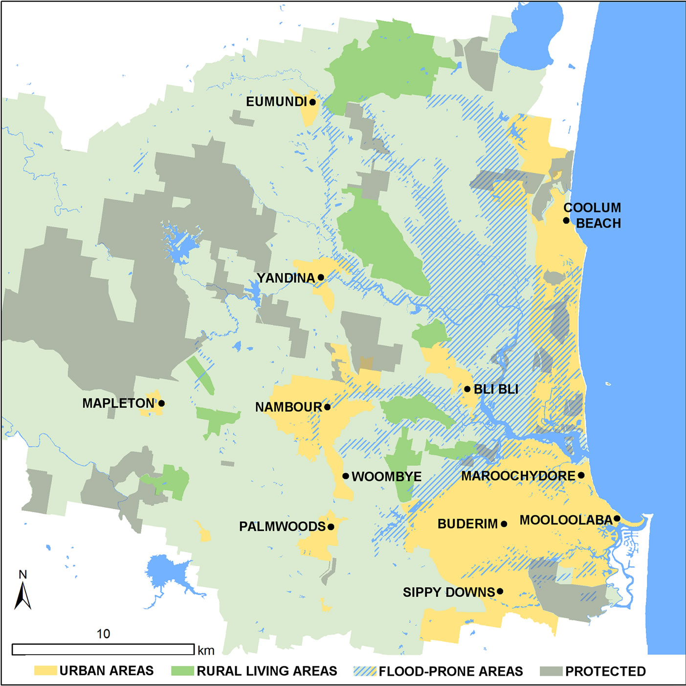
Figure 1. Diagram of Maroochy river catchment showing the location of the river, which is the blue river running inland north of Maroochydore, to the east of Bli Bli, then up to Yandina. The different colour codes represent the land uses.
tourism focused around nature-based activities, especially related to beach and river. It is a high socio-economic region, with average house sales of AU$626,000 (RPdata–www.rpdata.com.au). However, house prices are highly variable, with ocean or river front properties, selling for more than AU$1,500,000.
The aim of this study was to derive a value of the Maroochy River system to the local residents. A secondary issue was to identify how this value changed with different scenarios, e.g. poor water quality in the river resulting in the river not being valued by residents.
The Maroochy River is a dynamic natural asset and we have developed a conceptual model (Figure 2) to represent it. For example, further urban expansion may not lead to a static marginal increase in financial value of the Maroochy River to properties. This is because new dwellings would be built further from the river as the prime land has already been committed to urban development. More importantly, whilst the river contributes to property value, increased urban development and use of the River will decrease water quality and inturn decrease the value of the river (per capita) for its water users and properties close to the river. A decrease in water quality also means that there are greater costs in river restoration activities to improve water quality (Figure 2), and will also have adverse effects on the property values. This figure also shows how the analysis of this paper fits into the bigger picture of assessing the value of the Maroochy River. By presenting a dynamic model of the Maroochy River, we highlight the types of complex interactions that must be understood quantitatively, before a “whole-of-system” economic model of the Maroochy River can be built.
This paper focuses on one component of Figure 2, the financial value of property attributed to the Maroochy River. One would expect property values to be by far the largest financial benefit from the Maroochy River, particularly due to the canal frontages, views and the overall high socio-economic status of the Sunshine Coast. Calculating the contribution that the Maroochy River makes to the financial value of the properties around it is difficult. Firstly, there are many other confounding landscape features that contribute to the property values, such as the ocean, mountains (producing views of the ocean) and the city centre. Secondly, availability of reliable data for the region can be a challenge, particularly at the individual property level. For the Maroochy Shire, suitable GIS data sets were available from the Council, and covered all 28,000 properties in the vicinity of the Maroochy River. Collectively, the data sets contained information on size of the property, location, zoning of the land (resi-
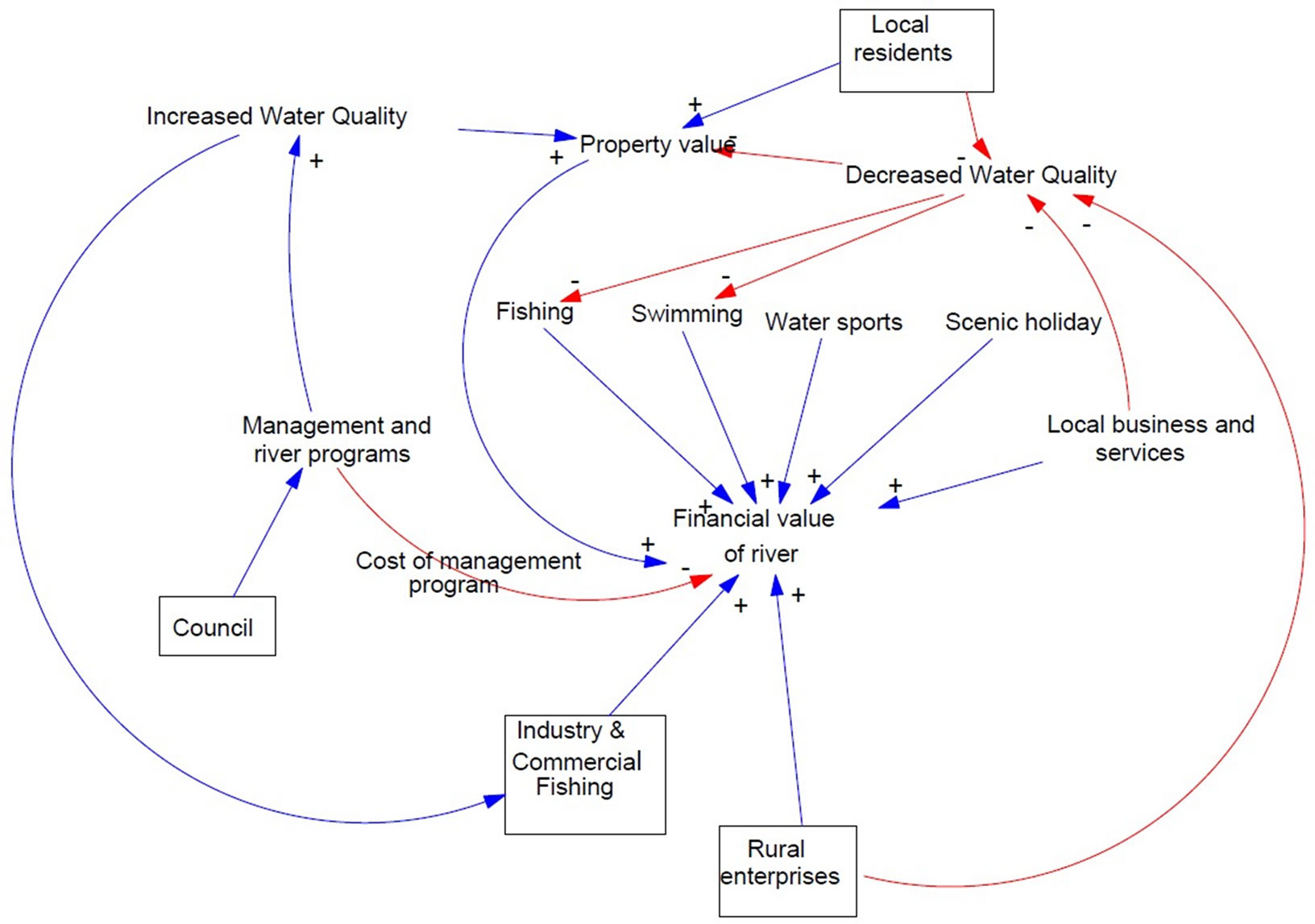
Figure 2. Dynamic relationship between water quality and financial value of the river, where the blue arrows (+) represent positive influences, and red arrows (-) represent negative influences.
ential, agriculture, commercial, units), land value (unimproved capital value), elevation. Other GIS layers provided information on property locations, and the location of the landscape features–ocean, rivers, towns, roads etc. Information on real estate sales prices of each property were obtained by RPdata (www.rpdata.com.au) and only contain information on properties that were sold in the last 5 years. This information only covered about 30 percent of properties.
We decided to base the analysis on unimproved capital value (UCV) rather than sales value of the properties, which was agreed upon by the Maroochy Shire Council. The main reason is that the value of the property, in relation to the natural assets (river, ocean) will be included in the land value (or UCV) rather than including confounding attributes such as the building itself. Additionally, there was inadequate sales data for the region over a set time period (ie. a thin housing market). UCV is the value of the land component of the property, as determined by the Queensland Valuer General, which is used by Maroochy Shire Council to calculate annual rates charged to the property owners. Since UCV is estimated through inspection, it doesn’t always represent the sale value of the vacant land, and doesn’t always capture the true value of environmental features to the resident. By using UCV we are able to ignore any confounding influences of building and landscaping (i.e. pools, etc.) that may be independent of location and proximity to the natural assets. A modelling approach needed to accommodate the 28,000 properties across the landscape, and the data set for these properties provided an excellent training set for the ANN developed for the analysis. For the case study, we focused on residential properties, and removed the commercial and agricultural properties from the original 28,000, leaving 26,500. The small number of commercial and agricultural properties (compared to residential) had highly variable UCV due to other variables (e.g. proximity to central business district) strongly affecting the UCV the council assesses these properties at. This made it very difficult to predict an economic value of these properties in relation to proximity, access or view of natural assets, and thuswas omitted from the analysis. Whilst distance to the Maroochy River was the key driver of the analysis of this paper, a model needed to accommodate other confounding effects. One of the purposes of the project working group, which included representatives from the Maroochy Shire Council, was to decide on variables that have the greatest impact on property value where there are data available. We agreed that the key variables were: location, distance to the ocean, elevation above sea level, distance to the river and streams, and area of the property. One would expect each of these variables to have some correlation with UCV, and the next section explores the strength of correlation. Other variables are also expected to impact UCV (e.g. adjoining busy roads or schools, availability of public transport, sewerage networks under properties). However, these were either not available or difficult to derive in a reliable form during the data preparation.
3. Application of an Artificial Neural Network
Considerable data preparation was required to consolidate the GIS and UCV databases for the Maroochy shire and to generate the variables used in the ANN. This included merging and reprojecting available data to match, as well as adding property value data to the relevant areas, using a Geodatabase. ArcGIS was used to generate: location (X,Y co-ordinates of the property centroid), the distance to coast, distance to major stream and stance to the main river. We included the main river as well as major streams in the analysis since the majority of properties are a considerable distance (>2 km) to the main river but are close to a major stream that feeds into the river. In some instances, close proximity to a major stream can have negative implications on a property value due to flood prone risks. Figure 3 shows some of the stages of analysis, to derive distance to coast and distance to streams using GIS methods. These were combined for this study. Table 1 contains a sample of the 26,500 data points used in the ANN after the data preparation phase.
An ANN is an information processing model inspired by the way the interconnected structure of the brain proc-
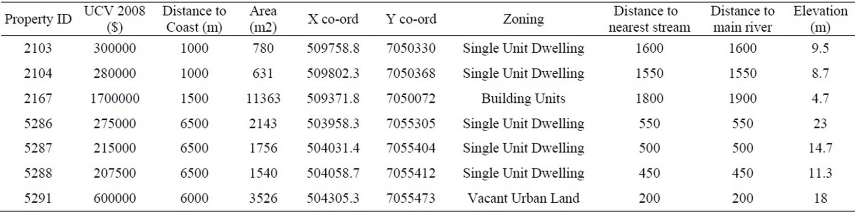
Table 1. Sample of data used for the ANN.
esses information. ANN’s are simplified mathematical models of biological neural networks. They consist of an interconnected group of artificial neurons and processes information using a connectionist approach to computation. In most cases an ANN is an adaptive system that changes its structure based on external or internal information that flows through the network during the learning phase. In more practical terms ANN’s are non-linear statistical data modelling tools. They can be used to model complex relationships between inputs and outputs or to find patterns in data. A widely used ANN structure is the multi-layer perceptron, which we have employed in this paper. It contains one input layer, two hidden layers and one output layer. Each layer employs several neurons and each neuron in the layer is connected to neurons in the adjacent layer through various weights. An illustration for the Maroochy case study is contained in Figure 4. Not all of the 30 neurons of hidden layer 1 and 15 neurons of hidden layer 2 are shown due to space limitations. The ANN was coded in NeuroSolutions 5. Twenty percent of the 26,500 properties in the dataset were used as cross validation, whilst the remaining 80 percent were used for the training set. The standard learning algorithm, back propagation, was used as the learning algorithm. Other parameters used in the ANN were: maximum epochs=12,000 where the mean square error of the cross validation set was minimal at this point; momentum=0.9; tolerance=0.0001; Tanh transfer function with beta=1.0; learning rate=0.1. We experimented with various combinations of number of neurons (5-100) and hidden layers (1-3) before arriving at the best combination for the analysis in terms of mean square error (MSE) for the cross validation data set. Whilst removing any of the input variables increased the MSE of the cross validation set, the contribution to the model did vary. When an ANN was fitted to each input variable to estimate UCV, the MSE varied from 0.00039 to 0.00045. The small difference between MSE of individual variables was likely due to large diversity of properties in the Maroochy shire, and the variables that influence their individual UCV. For example, for properties close to the ocean, ‘distance to coast’ was the most influential variable. UCV of large properties were influenced by the ‘area of property’ variable. This feature was also common to the ‘distance to river’, ‘location’, and ‘elevation’ variables. Zoning was a categorical variable, and was needed to separate out units from single unit dwellings, from large acre blocks, since UCV was calculated differently depending on the zoning. These reasons, along with the small MSE for each variable, were justification to include all variables selected by the Maroochy Shire Council. When all variables were included in the model, the MSE was 0.00032.
Correlation between actual UCV and those estimated using the ANN model was 0.62, and a scatter plot of the cross-validation data set is shown in Figure 5. A linear trend line is also shown as well as a one to one relationship (dotted line). The main deficiency of the ANN was the underestimation for high UCV, with an average error
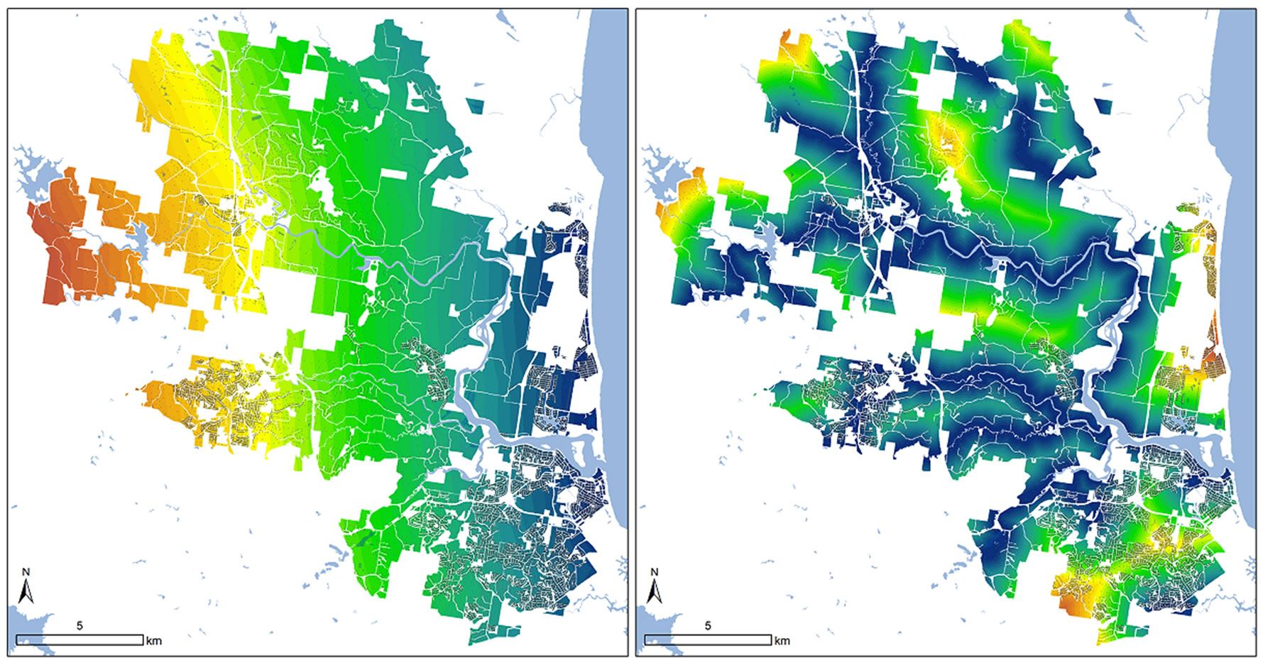
Figure 3. Data preparation-modelling of distances from ocean (left) and major stream (right), where blue represents closer distances and yellow/orange represents further distances.
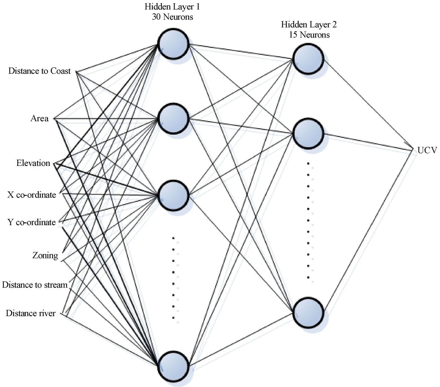
Figure 4. ANN architecture for Maroochy case study.
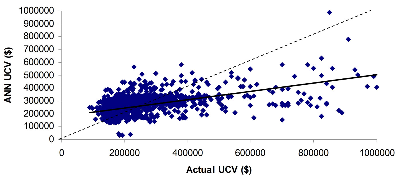
Figure 5. Relationship between actual UCV and those produced by the ANN for the cross-validation data.
of 39%. For the mainstream UCV values of AU$ 150,000 to AU$300,000 (with a median value of AU$ 197,000), underestimation was not a major problem, and the average error of estimation was 18%. Congestion of points between this range in Figure 5, makes it difficult to visually see the number points close to the trend line. A correlation of 0.62 and average error of 18%, would unlikely be high enough to use for the pur-pose of forecasting UCV’s for individual properties, particularly outside the current dataset. There are several other variables that the Valuer General accounts for when judging a property (e.g. closeness to main roads, intersections and public transport, major sewerage pipes under the property) which would have improved the correlation, though we were not able to accommodate in our current model. However, it was not important to include these other variables, since they were unlikely to have confounding impacts on the ‘distance to river and stream’ variables. The purpose the current model was to estimate the influence of the major environmental feature, the Maroochy River, on overall property values. Our priority was to capture that relationship as best as possible for the Maroochy dataset, whilst accommodating variables that would confound it (e.g. distance to ocean).
4. Application to Maroochy River Value and Scenarios
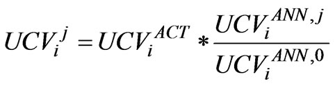
To estimate the value of the Maroochy River to property values, we needed to compare two scenarios: the current landscape as is, which we refer to as the base case; and the landscape with no river. The difference in property value between the two scenarios provides us with the estimated unimproved capital values with the river removed. To simulate the scenario with no river we allocated each property a 2.5km distance (minimum) to the main Maroochy River, and estimated the UCV using the ANN. The Maroochy Shire Council felt a 2.5km value is far enough from the river so that it does not influence UCV, which for the scenario would be analogous to not having a river. Since the ANN underestimated the actual UCV when the values were large, we needed to adjust the UCV’s produced by the ANN to produce a true representation of the value of the Maroochy River. We did this using the following formula:
where:
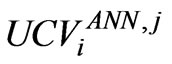
 = estimated UCV for property i in scenario j using the ANN after correcting for underestimation bias
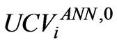
 =actual UCV for property i as per the raw data from the Maroochy council (base case),
  =
= 
 =raw UCV output from the ANN for property i in scenario j
 = raw UCV output from the ANN for property i in the base case scenario.
Let the scenarios be defined as follows:
Base case:- j =0 Main river removed:- j =1 Main river and main streams removed:- j =2. In this scenario each property is allocated a minimum distance of 2.5km to the nearest main stream.
The total unimproved capital value for all residential properties in the base case (with the river j =0) is AU$6,778,916,814, =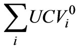 , which is summation of modelled UCV over all 26 500 residential properties in the Maroochy area. The first analysis was to remove the main river (Figure 6). By doing this, the total nonimproved capital value for all residential properties reduced to AU$5,880,347,570=
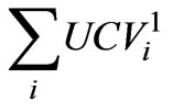 . This means the main section of the river is worth approximately AU$900,000,000 (AU$6,778,916,814 - AU$5,880,347, 570) to the residential property stock in the Maroochy region. There was some variability around this value depending on the ANN weights obtained during training, as each time the ANN is trained, a slightly different set of weights are obtained. Such variability led to an error bar of AU$900,000,000 plus or minus 22 percent. Figure 6 shows the value of the main river (scenario j =1) the across properties on a geographical basis, where the insert is the township of Maroochy. The colour codes represent the percentage of UCV remaining if the river was removed =
  /
/ *100. Areas in red and pink highlight properties where the main river is of greatest value, since they represent the greatest decrease in UCV with the river removed scenario (scenario j =1). These are generally properties closest to the river. Many of the properties in red are waterfront (canal) residents who have direct access for boating. In practice these properties sell for up to four times the price compared to properties without a canal frontage, so the ANN has predicted these instances very well. Some larger properties increased in value with scenario 1, and are due to removing the flood prone risks.
The second scenario (j =2) simulated the removal of the main Maroochy River and the main streams that feed into the main river. By doing this, the total non-improved capital value for all residential properties reduced to AU$5,828,577,742 = . This means the major streams (minus the main river) are worth about AU$52,000,000 (AU$5,880,347,570-AU$5,828,577,742) to residential properties. Actually, the main streams were found to have a negative impact on some properties (i.e. increased UCV from removing the streams, represented by dark green properties in Figure 7), because the streams created flood prone problems. Figure 7 colour codes represent the percentage of UCV remaining if the river and main streams were removed =
  /
/  *100. This an accurate representation of practice for most properties highlighted in dark green in Figure 7, which tend to be the larger low lying peri-urban areas. The scenarios highlight the capability of the ANN to accommodate the confounding relationships between variables such as elevation and distance to the river and ocean, as it can capture the negative implications of low lying land near the river.
The above capitalised values for each scenario can also be used to estimate rates income to Maroochy Shire Council, resulting from the river. Council uses a differential rating system based on UCV value of residential properties. We have simplified the analysis to provide the breadth of rate income council could derive from the Maroochy River based on the total changes in UCV expected by the ANN. To this end we assumed that all properties were in a range between AU$160,000 and AU$1 million and we have estimated the spread of council derived rates, due to the Maroochy River in Table 2. By estimating the annual rates to council resulting from the presence of the Maroochy River (Table 2), the Maroochy Shire Council will justify expenditure for protecting the ecosystem function of the river. This management program expenditure is highlighted in Figure 2 as part of the overall system of defining financial value of a river.
There are a broader range of planning and policy sce narios that the ANN for the Maroochy River could be
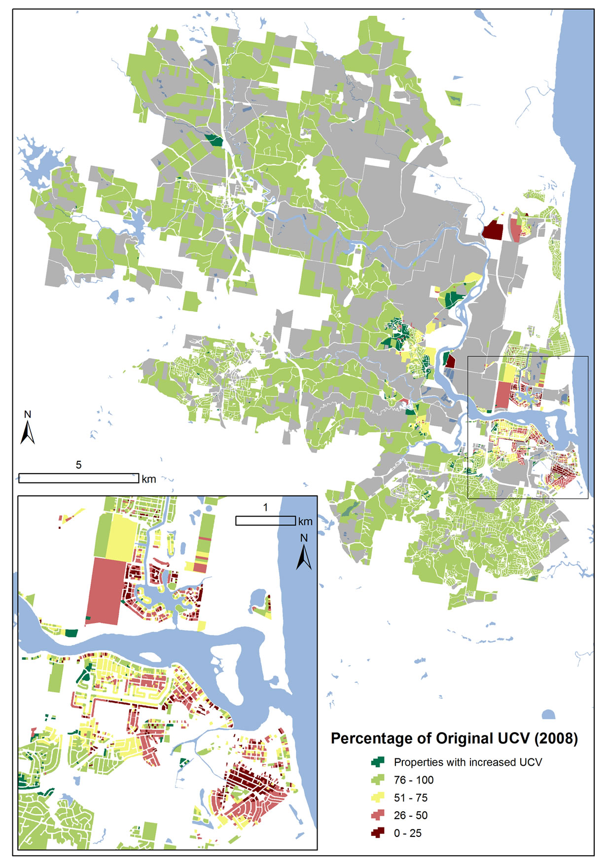
Figure 6. Spatial analysis of the impact of the Maroochy River on residential unimproved land values in Maroochy, based on removal of the main river.
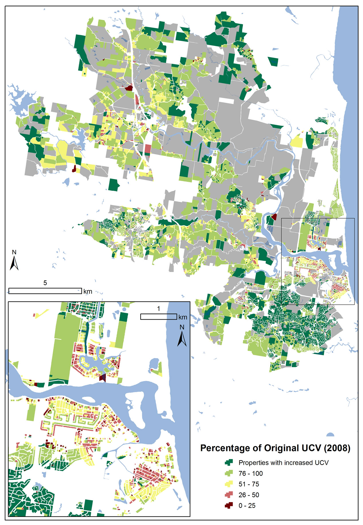
Figure 7. Spatial analysis of the impact of the Maroochy River on residential unimproved land values in Maroochy, based on removal of major stream and main river channel.
applied to in the future. This includes assessing the value of new residential property estates in a regional development plan for urban expansion, which would provide the Council with projections of future rates income. By applying the ANN to sales values as well as UCV, one can estimate the financial value of a property in terms of a relationship between building features and location. Such a capability would provide property developers with a means of tailoring housing stock designs in different locations (accommodating proximity to environmental assets) with market trends.
5. Conclusions
In this paper, we have addressed a novel application of assessing the financial value of a river to residential properties. It is also a novel application of ANN, which was shown to be a suitable method for estimating property value as a function of various landscape features, in the presence of a complete data set at property level.
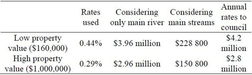
Table 2. Estimate of the possible range of Council residential rates derived from Maroochy River.
Whilst the ANN consistently underestimated large value of UCV, it was able to be corrected when applied to scenarios of economic value of the river to residents. The modelling approach was strongly welcomed by researchers and policy analysts, as it provided a credible value of Maroochy River for the first time without extensive primary data collection. By having a financial value of the river, the local River managers can go to the next step in justifying management expenditure in protecting the value of the river.
The existing analysis does have some challenges though. There is some room for improvement in accuracy of the model (correlation = 0.62), which can be done through introducing more variables such as proximity to amenities, busy roads, schools, and other features that impact land value. The use of UCV as an indicator of land value can also be questioned. It is the best indicator from the perspective of estimating financial income to the council through land rates, and is also suitable when a complete data set is needed. However, it is often not a true representative value of the sale price of the vacant land, as the sale price is usually higher than the UCV. Also, UCV’s of properties are often estimated using expert ‘valuer’ opinions. There is limited data available on sales of vacant land, as more properties are sold with a house, though the limited sales information could be used to calibrate UCV’s if there is sufficient representation. These opportunities will be investigated as part of future research.
The analysis of this paper is one step towards estimating the full economic value of the Maroochy River, and other research is being conducted to estimate contributions from tourism, water sports, industry and agriculture [34]. The Maroochy Shire council, like many government bodies, wish to better understand the relationship between environmental and economic value and hence ensure more effective management of its environmental assets into the future. A next major step of the research will be turn the framework of Figure 2 into dynamic systems model linking the modelling work of this paper with models representing other components of Figure 2.
6. Acknowledgements
We thank the Maroochy Shire project working group, led by Damian McGarry, who provided the wide range of data and analysis for the analysis. We also thank Dr Heinz Schandl of CSIRO for suggestions to improve the paper.
REFERENCES
- C. Lee and P. Linneman, “Dynamics of the greenbelt amenity effect on the land market-The case of Seoul’s greenbelt,” Real Estate Economics, Vol. 26, pp. 107–129, 1998.
- L. J. Pearson, C. Tisdell and A. T. Lisle, “The impact of Noosa national park on surrounding property values: An application of the hedonic price method,” Economic Analysis and Policy, Vol. 32, No. 2, pp. 155–171, 2002.
- N. Hanley, R. E. Wright and B. Alvarez-Farizo, “Estimating the economic value of improvements in river ecology using choice experiments: An application to the water framework directive,” Journal of Environmental Management, Vol. 78, pp. 183–193, 2006.
- H. Chen, N. Chang and D. Shaw, “Valuation of in-stream water quality improvement via fuzzy contingent valuation method,” Stochastic Environmental Research Risk Assessment, Vol. 19, pp. 158–171, 2005.
- R. A. Kramer and J. I. Eisen-Hecht, “Estimating the economic value of water quality protection in the Catawba River basin,” Water Resources Research, Vol. 30, No. 9, pp. 1182, 2002.
- R. C. Mitchell and R. T. Carson, “Using surveys to value public goods: The contingent valuation method,” Resources of the Future, Washington, D.C, 1989.
- M. K. Alam and D. Marinova, “Measuring the total value of a river cleanup,” Water Science and Technology, Vol. 48, pp. 149–156, 2003.
- R. S. Rosenberger and J. B. Loomis, “Benefit transfer of outdoor recreation use values. A technical Document Supporting the Forest Service Strategic Plan,” Gen. Tech. Rep. RMRS-GTR-72. Fort Collins, CO: U.S. Department of Agriculture, Forest Service, Rocky Mountain Research Station, pp. 59, 2001.
- G. Van Houtven, J. Powers and S. K. Pattanayak, “Valuing water quality improvements in the United States using meta-analysis: Is the glass half full or half empty for national policy analysis?” Resource and Energy Economics, Vol. 29, pp. 206–228, 2007.
- S. Rosen, “Hedonic prices and implicit markets: Product differentiation in perfect competition,” Journal of Political Economy, Vol. 82, No. 1, pp. 34–55, 1974.
- S. D. Shultz, “The use of census data for hedonic price estimates of open-space amenities and land use,” Journal of Real Estate Finance and Economics, Vol. 22, No. 2/3, pp. 239–252, 2001.
- G. Acharya and B. L. Lewis, “Valuing open space and landuse patterns in urban watersheds,” Journal of Real Estate Finance and Economics, Vol. 22, pp. 221–237, 2001.
- B. L. Mahan, S. Polasky and R. M. Adams, “Valuing urban wetlands: A property price approach,” Journal of Land Economics, Vol. 76, pp. 100–113, 2000.
- E. D. Benson, J. L. Hansen, J. Arthur, L. Schwartz, G. T. Smersh, “Pricing residential amenities: The value of a view,” Journal of Real Estate Finance and Economics, Vol. 16, pp. 55–73, 1998.
- B. Colby and S. Wishart, “Riparian areas generate property value premium for landowners,” Working paper, University of Arizona College of Agriculture and Life Sciences, Department of Agricultural and Resource Economics, 2002.
- K. Boyle and L. Taylor, “Does the measurement of property and structural characteristics affect estimated implicit prices for environmental amenities in a hedonic model?” Journal of Real Estate Finance and Economics, Vol. 22, No. 2/3, pp. 303–318, 2001.
- L. Tyrvainen, “The amenity value of the urban forest: an application of the hedonic pricing method,” Landscape and Urban Planning, Vol. 37, pp. 211–222, 1997.
- W. A. Donnelly, “Hedonic price analysis of the effect of a floodplain on property values,” Journal of the American Water Resources Association, Vol. 25, No. 3, pp. 581–586, 2007.
- S. Sengupta and D. E. Osgood, “The value of remoteness: A hedonic estimation of ranchette prices,” Ecological Economics, Vol. 44, pp. 91–103, 2003.
- B. Fraser and G. Spencer, “The value of an ocean view: An example of hedonic property amenity valuation,” Australian Geographical Studies, Vol. 36, No. 1, pp. 94–98, 1998.
- J. Luttik, “The value of trees, water and open space as reflected by house prices in the Netherlands,” Landscape and Urban Planning, Vol. 48, pp. 161–167, 2000.
- C. Bastian, D. McLeod, M. Germino, W. Reiners and B. Blasko, “Environmental amenities and agricultural land values: A hedonic model using geographical information systems data,” Ecological Economics, Vol. 40, pp. 337–349, 2002.
- I. R. Lake, A. Lovett, I. J. Bateman, I. H. Langford, “Modelling environmental influences on property prices
- in an urban environment,” Computers, Environment and
- Urban Systems, Vol. 22, pp. 121–136, 1998.
- A. Freeman and I. I. I. Myrick, “The measurement of environmental and resource values,” Theory and Methods, Resources for the Future, 1997.
- D. W. Pearce and A. Markandya, “Environmental policy benefits: Monetary valuation,” Organisation for Economic Co-operation and Development, Paris, 1989.
- J. A. Anderson, “An Introduction to Neural Networks”. M. I. T. Press, 1995.
- T. Khanna, “Foundations of Neural Networks,” Addison-Wesley, 1990.
- H. Selim, “Determinants of house prices in Turkey: Hedonic regression versus artificial neural network,” Expert Systems with Applications, In press, 2008.
- R. O. Strobl and F. Forte, “Artificial neural network exploration of the influential factors in drainage network derivation,” Hydrological Processes, Vol. 21, pp. 2965– 2978, 2007.
- Y. Miao, D. J. Mulla, and P. C. Robert, “Identifying important factors influencing corn yield and grain quality variability using artificial neural networks,” Precision Agriculture, Vol. 7, pp. 117–135, 2006.
- J. C. Ingram, T. P. Dawson, R. J. Whittaker, “Mapping tropical forest structure in southeastern Madagascar using remote sensing and artificial neural networks,” Remote Sensing of Environment, Vol. 94, pp. 491–507, 2004.
- N. Garcia, M. Gamez and E. Alfaro, “ANN+GIS: An automated system for property valuation,” Neurocomputing, Vol. 71, pp. 733–742, 2008.
- P. S. Jarvis, I. D. Wilson and S. E. Kemp, “The application of a new attribute selection technique to the forecasting of housing value using dependence modelling,” Neural Computing and Applications, Vol. 15, pp. 136–153, 2006.
- L. J. Pearson, A. J. Higgins, L. Laredo and S. Whitten, “Maroochy River Value Project,” Final Report submitted to the Sunshine Coast Regional Council, 2008.