Journal of Software Engineering and Applications
Vol.6 No.4A(2013), Article ID:30072,7 pages DOI:10.4236/jsea.2013.64A002
Lognormal Process Software Reliability Modeling with Testing-Effort
![]()
Department of Social Management Engineering, Graduate School of Engineering, Tottori University, Tottori, Japan.
Email: ino@sse.tottori-u.ac.jp, yamada@sse.tottori-u.ac.jp
Copyright © 2013 Shinji Inoue, Shigeru Yamada. This is an open access article distributed under the Creative Commons Attribution License, which permits unrestricted use, distribution, and reproduction in any medium, provided the original work is properly cited.
Received December 26th, 2012; revised January 29th, 2013; accepted February 6th, 2013
Keywords: Software Reliability Growth Model; Lognormal Process; Testing-Effort Function; Software Reliability Assessment Measures; Goodness-of-Fit
ABSTRACT
We propose a software reliability growth model with testing-effort based on a continuous-state space stochastic process, such as a lognormal process, and conduct its goodness-of-fit evaluation. We also discuss a parameter estimation method of our model. Then, we derive several software reliability assessment measures by the probability distribution of its solution process, and compare our model with existing continuous-state space software reliability growth models in terms of the mean square error and the Akaike’s information criterion by using actual fault count data.
1. Introduction
Quantitative software reliability assessment is one of the important activities to produce reliable software systems. A software reliability growth model (abbreviated as SRGM) [1,2] is known as a useful mathematical tool for assessing software reliability quantitatively. The SRGM can describe the software fault-detection phenomenon or the software failure-occurrence phenomenon in the testing or operational phase by applying stochastic and statistical theories. Especially, a nonhomogeneous Poisson process (abbreviated as NHPP) [3,4], which describes the faultdetection phenomenon as a discrete-state space, is often applied in software reliability growth modeling by supposing an appropriate mean value function of the NHPP. Accordingly, the NHPP model is utilized for quantitative software reliability assessment in many software houses and computer manufacturers from the view point of the high applicability and simplicity of the model structure of an NHPP.
In contrast with discrete-state space SRGMs, such as well-known NHPP models [5], there are continuousstate space SRGMs to assess software reliability for large scale software systems. Specifically, Yamada et al. [6] discussed a framework for the continuous-state space software reliability growth modeling based on a stochastic differential equation of Itô type, and compared the continuous-state space SRGM with the NHPP models. Recently, Yamada et al. [7] and Lee et al. [8] proposed several type of the continuous-state space SRGMs based on stochastic differential equations of Itô type, such as exponential, delayed S-shaped, inflection S-shaped stochastic differential equation models, by characterizing the fault-detection rate per unit time per one fault, respectively.
However, these continuous-state space SRGMs have not taken the effect of testing-effort into consideration in software reliability assessment. The testing-effort, such as the number of executed test-cases, testing-coverage, and CPU hours expended in the testing phase, is well known as one of the most important factors being related to the software reliability growth process [9]. Under the above background, there is necessity to discuss a testingeffort dependent SRGM on a continuous-state space for the purpose of developing a more plausible continuous-state space SRGM.
This paper proposes a continuous-state space software reliability growth model with the testing-effort factor by applying a mathematical technique of stochastic differrential equations of Itô type, and conducts goodnessof-fit comparisons of our model with existing continuous-state space SRGMs. Concretely, we extend a basic differential equation describing the behavior of the cumulative number of detected faults to a stochastic differential equation of Itô type by considering with the testing-effort factor, and derive its solution process which represents the fault-detection process. Then, we discuss estimation methods for unknown parameters in our model. And we then compare our model with existing continuous-state space SRGMs in terms of the mean square error (MSE) [5] and Akaike’s information criterion (AIC) [10]. Finally, we derive several software reliability assessment measures by the probability distribution of the solution process, and show numerical examples for software reliability assessment measures derived from our model by using actual fault counting data.
2. Basic Modeling Framework
We discuss a framework of continuous-state space software reliability growth modeling [6]. Letting  be a random variable which represents the number of faults detected up to time t. From the common assumptions for software reliability growth modeling, that is, the instantaneous number of detected faults at time t depends on the residual number of undetected faults at time t [1,2,5], we have the following linear differential equation:
 (1)
(1)
where b(t) indicates the fault-detection rate at testing-time t and is assumed to be a non-negative function, and a the initial fault content in the software system. Equation (1) describes the behavior of the decrement of the fault content in the software system.
Especially, in the large-scale software development, a fault-detection process in an actual testing phase is influenced by several uncertain testing-factors, such as testing-skill, debugging-environment. Accordingly, we should take these factors into consideration in software reliability growth modeling. Therefore, we extend Equation (1) to the following equation:
 , (2)
, (2)
where  is a noise that exhibits an irregular fluctuation. For the purpose of making its solution a Markov process, we assume that
  in Equation (2) has
 , (3)
, (3)
where ![]() indicates a positive constant representing magnitude of the irregular fluctuation and
indicates a positive constant representing magnitude of the irregular fluctuation and ![]() a standardized Gaussian white noise.
a standardized Gaussian white noise.
We transform Equation (2) into the following stochastic differential equation of Itô type:
 (4)
(4)
where W(t) is a one-dimensional Wiener process which is formally defined as an integration of the white noise  with respect to time t. The Wiener process W(t) is called a Gaussian process, and has the following properties:
 (a)
(a)
 (b)
(b)
 (c)
(c)
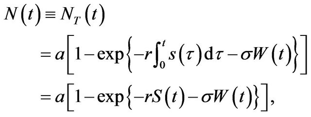
where Pr[A] and E[·] represent the probability of the event A and the expectation, respectively. Next, we derive a solution process N(t) by using the Itô’s formula. The solution process N(t) can be derived as
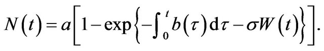 (5)
(5)
Equation (5) implies that the solution process N(t) obeys a geometric Brownian motion or a lognormal process [11]. And the transition probability distribution of the solution process N(t) is derived as
 (6)
(6)
consequently, by the properties (a)-(c) and the assumption that W(t) is a Gaussian process.  in Equation (6) indicates a standard normal distribution defined as
 (7)
(7)
By giving an appropriate function b(t) in Equation (5), we can derive several SRGM’s. Yamada et al. [7] and Lee et al. [8] proposed several lognormal process models, in which the fault-detection rates b(t) follow the basic modeling assumptions of the well-known NHPP model, such as the delayed S-shaped [12] and inflection Sshaped [13] SRGMs, based on the modeling framework [6] mentioned in this section
3. Lognormal Process SRGM with Testing-Effort
We develop a continuous-state space SRGM with the effect of testing-effort factor based on stochastic differential equations which follow the lognormal process. The testing-effort, such as the number of executed test-cases, testing-coverage, and CPU hours, is one of the important factors influencing on the software reliability growth process in an actual testing-phase. Therefore, the testing-effort should be taken into consideration in continuous-state space software reliability growth modeling.
3.1. Modeling
For developing a continuous-state space SRGM with the effect of the testing-effort factor, we characterize b(t) in Equation (5) as follows:
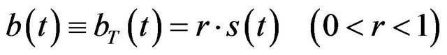 , (8)
, (8)
where r represents the fault-detection rate per expended testing-effort at testing time t and s(t)(![]() dS(t)/dt) is the amount of the testing-effort expended at arbitrary testing time t. In Equation (8), we assume that the fault-detection rate at testing-time t depends on the instantaneous testing-effort expenditures [9]. That means, the testing-team can detect or remove more software faults when the software development manager decides to expend more testing-effort to detect or remove software fault. Based on the framework of continuous-state space software reliability growth modeling [6], we can obtain the following solution process:
dS(t)/dt) is the amount of the testing-effort expended at arbitrary testing time t. In Equation (8), we assume that the fault-detection rate at testing-time t depends on the instantaneous testing-effort expenditures [9]. That means, the testing-team can detect or remove more software faults when the software development manager decides to expend more testing-effort to detect or remove software fault. Based on the framework of continuous-state space software reliability growth modeling [6], we can obtain the following solution process:
 (9)
(9)
The transition probability distribution function of the solution process in Equation (9) can be derived as
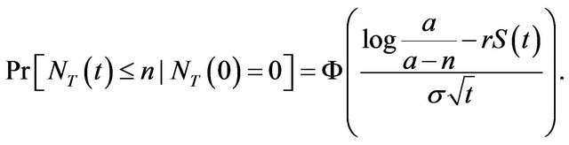 (10)
(10)
We should specify the testing-effort function s(t) in Equation (8) to utilize the solution process  in Equation (9) as an SRGM.
3.2. Testing-Effort Function
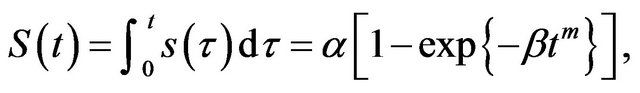
We need to specify a suitable function for the s(t) in Equation (8). In this paper we describe the time-dependent behavior of testing-effort expenditures in the testing-phase by using a Weibull curve function, that is,
 (11)
(11)
Then, we have
 (12)
(12)
where ![]() is the total amount of testing-effort expenditures,
is the total amount of testing-effort expenditures,  the scale parameter, and m the shape parameter characterizing the shape of the testing-effort function. The Weibull curve function has a useful property to describe the time-dependent behavior of the expended testing-effort expenditures in the testing-phase approximately because of its flexibility. For examples, we can obtain the exponential curves when m = 1 in Equations (11) and (12). And when m = 2, we can derive Rayleigh curves. That is, the Weibull curve function is a general type model, which includes the exponential and Rayleigh curve functions.
4. Parameter Estimation
We discuss estimation methods of unknown parameters of the testing-effort function in Equation (11) and the solution process in Equation (9), respectively. Now we suppose that K data pairs 
 with respect to the total number of faults,
  detected during the time-interval
  and the amount of testing-effort expenditures,
  , expended at
 ![]() are observed.
are observed.
4.1. For the Testing-Effort Function
Regarding a parameter estimation method for the testing-effort function in Equation (11), we use a method of least squares. First we can obtain the following equation by taking the natural logarithm of Equation (11):
 (13)
(13)
Then, the sum of the squares of vertical distances from the data points to the estimated values is derived as
 (14)
(14)
by using Equation (13). The estimations  and
and  for the parameters
  and
and ![]() minimizing
minimizing
 in Equation (14) can be obtained by solving the following simultaneous equations:
 (15)
(15)
4.2. For the Solution Process
Next we discuss a parameter estimation method for the solution process in Equation (9) by using the method of maximum-likelihood. Let us denote the joint probability distribution function of the process  as
as
 (16)
(16)
and also denote its density as
 (17)
(17)
Then, we can derive the likelihood function l for the observed data pairs  as follows:
 (18)
(18)
For convenience in the mathematical manipulations, we use the following logarithmic likelihood function:
 (19)
(19)
The likelihood function l in Equation (18) can be written as the following equation by using the Bayes’ formula and a Markov property:
 (20)
(20)
where  is the conditional probability density under the condition of
  The transition density
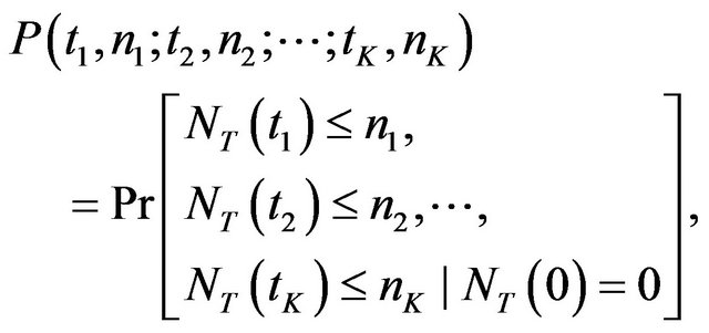
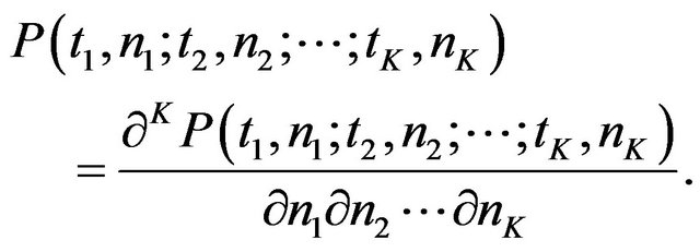
  in Equation (20) can be obtained by partially differentiating the following transition probability of
  under the condition
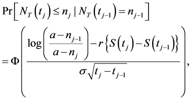 (21)
(21)
with respect to  Consequently, the likelihood function l in Equation (20) can be rewritten as
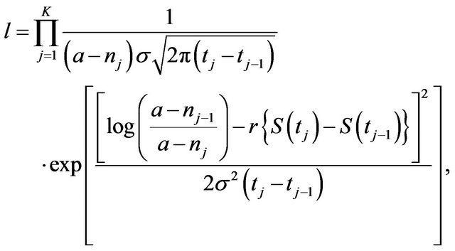 (22)
(22)
and the logarithmic likelihood function is derived as
 (23)
(23)
Then, we can obtain the maximum likelihood estimations ![]() and
and  for the parameters
 ![]() and
and ![]() in Equation (9) by solving the following simultaneous likelihood equations numerically:
in Equation (9) by solving the following simultaneous likelihood equations numerically:
 (24)
(24)
5. Software Reliability Assessment Measures
We derive several software reliability assessment measures, which are useful for quantitative assessment of software reliability. Especially, we derive instantaneous and cumulative MTBF’s in this paper.
5.1. Instantaneous MTBF
We discuss an instantaneous MTBF (mean time between software failures or fault-detections) which has been used as one of the substitution for the usual MTBF. An instantaneous MTBF is approximately derived by
 (25)
(25)
We need to derive , which represents the expected number of faults detected up to arbitrary testing time t, to obtain
  in Equation (25). By the Wiener process W(t) ~ N(0,t), the expected number of faults detected up to arbitrary testing time t is obtained as
 (26)
(26)
Since the Wiener process has the independent increment property W(t) and dW(t) are statistically independent with each other, and E[dW(t)] = 0,  in Equation (25) is finally derived as
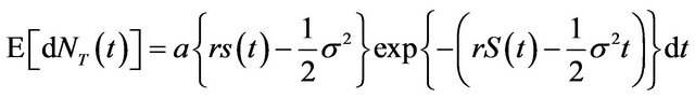 (27)
(27)
The instantaneous MTBF in Equation (25) can be calculated by substituting Equation (27) into Equation (25).
5.2. Cumulative MTBF
A cumulative MTBF is also the substitution for the usual MTBF. The cumulative MTBF is approximately derived as
 (28)
(28)
If the instantaneous MTBF in Equation (25) and the cumulative MTBF in Equation (28) take on a large value, respectively, then it enables us to decide that the software system becomes more reliable.
6. Model Comparisons
We show results of goodness-of-fit comparisons of our model with other continuous-state space SRGMs [6-8], such as exponential, delayed S-shaped, and inflection S-shaped stochastic differential equations, in terms of the mean square errors (MSE) [5] and Akaike’s Information Criterion (AIC) [10]. Regarding the goodness-of-fit comparisons, we use two actual data sets [14] named as DS1 and DS2, respectively. DS1 and DS2 indicate an Sshaped and exponential reliability growth curves, respectively.
The MSE [5] is obtained by dividing the sum of squared errors between the observed and estimated cumulative numbers of detected faults,  and
and  during
  respectively, by the sample number of observed data. Assuming that K data pairs
 are observed, we can formulate the MSE as
 (29)
(29)
where  denotes the estimated value of the expected cumulative number of faults by arbitrary testing time
![]() . Accordingly, the model which indicates the smallest MSE fits best to the observed data set than other models.
. Accordingly, the model which indicates the smallest MSE fits best to the observed data set than other models.
The AIC [10] is known as a goodness-of-fit evaluation criterion considering the number of model parameter. The AIC is given by
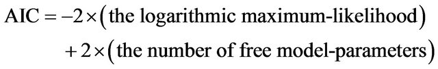 , (30)
We should note that the AIC values themselves are not significant. The absolute value of difference among their values is significant. We can judge that the model indicating the smallest AIC fits best to the actual data set if their differences are greater than or equal to 1. If the differences are less than 1, there are no significant.
Table 1 shows the results of model comparisons based on the MSE and the AIC, respectively. The model comparisons based on the AIC is not significant only for DS2, however, we can see that our model improves a performance of the MSE and the AIC respectively, compared with other continuous-state space SRGMs discussed in this paper.
Table 1. Results of model comparisons.
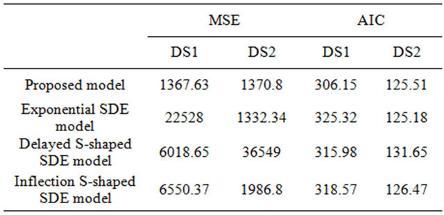
(SDE: stochastic differential equation).
7. Numerical Examples
We show numerical examples by using testing-effort data recorded along with detected fault counting data collected from the actual testing. In this testing, 1301 fault are totally detected and 1846.92 (testing hours) are totally expended as the testing-effort within 35 months [14].
Figure 1 shows the estimated testing-effort function ![]() in Equation (11), in which the parameter estimates as
in Equation (11), in which the parameter estimates as ,
,  , and
, and . As we can see, the actual time-dependent behaviour of the instantaneous testing-effort expenditures is observed on the discrete-time, and is quite oscillatory. Although it is very difficult to describe completely such behaviour by a mathematical model, the Weibull curve function in Equation (11) enables us to describe the time-dependent behaviour approximately and smoothly on the continuous-time function. Figure 2 shows the estimated expected number of detected faults in Equation (26), where the parameter estimates in
  are obtained as
 ,
,  , and
, and . Furthermore, Figure 3 shows the time-dependent behavior of the estimated two types of the substitutions of the MTBF, such as instantaneous and cumulative MTBFs in Equations (25) and (28), respectively. We should note that getting larger instantaneous or cumulative MTBF indicates growing the software reliability. From Figure 3, we can see that the software reliability decreases in the early testing period because the estimated software fault-detection rate is getting larger in the early testing period due to the model structure. And then, the software reliability grows as the testing procedures go on because the fault-detection rate is getting decrease and the residual fault content is also getting decrease. We note that the time-dependent behaviour of the instantaneous and cumulative MTBFs are different each other due to approximation methods. The instantaneous MTBF responds sensitively to the number of software faults detected at testing-time t because the instantaneous MTBF does not
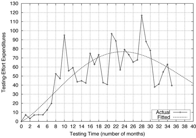
Figure 1. Estimated testing-effort function.
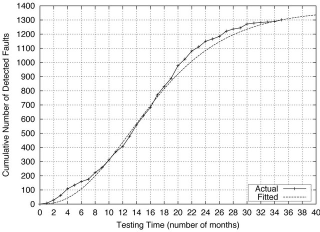
Figure 2. Estimated expected number of detected faults.
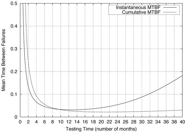
Figure 3. Estimated instantaneous and cumulative MTBFs.
incorporate information of the past software reliability growth process as shown in Equation (25). We can estimate the instantaneous MTBF at the termination time of the testing,  , to be about 0.1297 (about 4.5 months), and also, the cumulative MTBF,
  , to be about 0.0269 (about 0.9 months).
8. Concluding Remarks
We have discussed a continuous-state space SRGM with the effect of testing-effort by using a mathematical technique of stochastic differential equations and its parameters estimation methods. Then, we have compared performance in software reliability measurement of our model with existing continuous-state space SRGMs in terms of the MSE and the AIC by using actual data, respectively. Finally, we have also shown numerical illustrations for the software reliability assessment measures, such as the instantaneous and cumulative MTBFs.
We believe that software developing managers can get information on a relationship between the attained software reliability and the testing-effort expenditures by using our software reliability growth model. And our model also enables software development managers to decide how much testing-effort are expended to attain a reliability objective. Further studies are needed to examine the validity of our model for practical applications by using many observed data.
9. Acknowledgements
The second author is supported in part by the Grant-inAid for Scientific Research (C), Grant No. 22510150, from the Ministry of Education, Culture, Sports, Science and Technology of Japan.
REFERENCES
- J. D. Musa, D. Iannio and K. Okumoto, “Software Reliability: Measurement, Prediction, Application,” McGraw- Hill, New York, 1987.
- H. Pham, “Software Reliability,” Springer-Verlag, Singapore City, 2000.
- S. Osaki, “Applied Stochastic System Modeling,” SpringerVerlag, Berlin-Heidelberg, 1992. doi:10.1007/978-3-642-84681-6
- K. S. Trivedi, “Probability and Statistics with Reliability, Queueing and Computer Science Applications,” John Wiley & Sons, New York, 2002.
- S. Yamada, “Software Reliability Models,” In: S. Osaki, Ed., Stochastic Models in Reliability and Maintenance, Springer-Verlag, Berlin-Heidelberg, 2002, pp. 253-280. doi:10.1007/978-3-540-24808-8_10
- S. Yamada, M. Kimura, H. Tanaka and S. Osaki, “Software Reliability Measurement and Assessment with Stochastic Differential Equations,” IEICE Transactions on Fundamentals of Electronics, and Computer Sciences, Vol. E77-A, No. 1, 1994, pp. 109-116.
- S. Yamada, A. Nishigaki and M. Kimura, “A Stochastic Differential Equation Model for Software Reliability Assessment and Its Goodness-of-Fit,” International Journal of Reliability and Applications, Vol. 4, No. 1, 2003, pp. 1- 11.
- C. H. Lee, Y. T. Kim and D. H. Park, “S-shaped Software Reliability Growth Models Derived from Stochastic Differential Equations,” IIE Transactions, Vol. 36, No. 12, 2004, pp. 1193-1199. doi:10.1080/07408170490507792
- S. Yamada, H. Ohtera and H. Narihisa, “Software Reliability Growth Models with Testing-Effort,” IEEE Transactions on Reliability, Vol. R-35, No. 1, 1986, pp. 19-23. doi:10.1109/TR.1986.4335332
- H. Akaike, “A New Look at the Statistical Model Identification,” IEEE Transactions on Automatic Control, Vol. AC-19, No. 6, 1974, pp. 716-723. doi:10.1109/TAC.1974.1100705
- B. Øksendal, “Stochastic Differential Equations: An Introduction with Applications,” Springer-Verlag, BerlinHeidelberg, 1985.
- S. Yamada, M. Ohba and S. Osaki, “S-Shaped Software Reliability Growth Models and Their Applications,” IEEE Transactions on Reliability, Vol. R-33, No. 4, 1984, pp. 289-292. doi:10.1109/TR.1984.5221826
- M. Ohba, “Inflection S-Shaped Software Reliability Growth Model,” In: S. Osaki and Y. Hatoyama, Eds., Stochastic Models in Reliability Theory, Springer-Verlag, Berlin, 1984, pp. 144-165. doi:10.1007/978-3-642-45587-2_10
- W. D. Brooks and R. W. Motley, “Analysis of Discrete Software Reliability Models,” Technical Report RADCTR-80-84, Rome Air Development Center, New York, 1974.