Intelligent Information Management
Vol.5 No.3(2013), Article ID:31740,11 pages DOI:10.4236/iim.2013.53008
Estimation of Generalized Pareto under an Adaptive Type-II Progressive Censoring*
1Mathematics Department, Faculty of Science, A1-Azhar University, Nasr-City, Cairo, Egypt
2Faculty of Science, Islamic University, Madinah, Saudi Arabia
3Mathematics Department, Sohag University, Sohag, Egypt
Email: Rashadmath@Yahoo.com
Copyright © 2013 Mohamed A. W. Mahmoud et al. This is an open access article distributed under the Creative Commons Attribution License, which permits unrestricted use, distribution, and reproduction in any medium, provided the original work is properly cited.
Received January 21, 2013; revised February 27, 2013; accepted April 1, 2013
Keywords: Generalized Pareto (GP) Distribution; An Adaptive Type-II Progressive Censoring Scheme; Bayesian and Non-Bayesian Estimations; Gibbs and Metropolis Sampler; Bootstrap
ABSTRACT
In this paper, based on a new type of censoring scheme called an adaptive Type-II progressive censoring scheme introduce by Ng, et al. [1], Naval Research Logistics is considered. Based on this type of censoring the maximum likelihood estimation (MLE), Bayes estimation, and parametric bootstrap method are used for estimating the unknown parameters. Also, we propose to apply Markov chain Monte Carlo (MCMC) technique to carry out a Bayesian estimation procedure and in turn calculate the credible intervals. Point estimation and confidence intervals based on maximum likelihood and bootstrap method are also proposed. The approximate Bayes estimators obtained under the assumptions of non-informative priors, are compared with the maximum likelihood estimators. Numerical examples using real data set are presented to illustrate the methods of inference developed here. Finally, the maximum likelihood, bootstrap and the different Bayes estimates are compared via a Monte Carlo simulation study.
1. Introduction
In life testing and reliability studies, the experimenter may not always obtain complete information on failure times for all experimental units. Data obtained from such experiments are called censored data. Reducing the total test time and the associated cost is one of the major reasons for censoring. A censoring scheme, which can balance between, total time spent for the experiment, number of units used in the experiment and the efficiency of statistical inference based on the results of the experiment, is desirable. The most common censoring schemes are Type-I (time) censoring, where the life testing experiment will be terminated at a prescribed time T, and TypeII (failure) censoring, where the life testing experiment will be terminated upon the r-th (r is pre-fixed) failure. However, the conventional Type-I and Type-II censoring schemes do not have the flexibility of allowing removal of units at points other than the terminal point of the experiment. Because of this lack of flexibility, a more general censoring scheme called progressive Type-II right censoring has been introduced. Briefly, it can be described as follows: Consider an experiment in which n units are placed on a life testing experiment. At the time of the first failure,  units are randomly removed from the remaining
  surviving units. Similarly, at the time of the second failure,
  units from the remaining
  units are randomly removed. The test continues until the
  -th failure at which time, all the remaining
 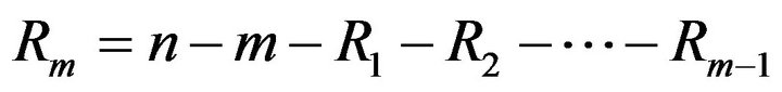 units are removed. The
  are fixed prior to the study. We note that prior to the experiment in the progressive Type-II right censoring, an integer
  is determined and the progressive Type-II censoring scheme
  with
with
 and
and  is specified. During the experiment, the i-th failure is observed and immediately after the failure, Ri functioning items are randomly removed from the test. We denote the m completely observed (ordered) lifetimes by
 , which are the observed progressively Type-II right censored sample. For convenience, we will suppress the censoring scheme in the notation of the
 ’s. We also denote the observed values of such a progressively Type-II right censored sample by
  Readers may refer to Balakrishnan [2] and Balakrishnan and Aggarwala [3] for extensive reviews of the literature on progressive censoring.
Recently, Ng, et al. [1] suggested an adaptive Type-II progressive censoring, where we allow  to depend on the failure times so that the effective sample size is always m, which is fixed in advance. A properly planned adaptive progressively censored life testing experiment can save both the total test time and the cost induced by failure of the units and increase the efficiency of statistical analysis.
Arandom variable X is said to have generalized Pareto (GP) distribution, if its probability density function (pdf) is given by
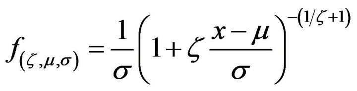
where  and
and . For convenience, we reparametrized this distribution by defining
 and
and . Therefore,
 (1)
(1)
The cumulative distribution function (cdf) is defined by
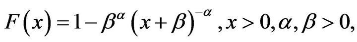 (2)
(2)
Here  and
and  are the shape and scale parameters, respectively. It is also well known that this distribution has decreasing failure rate property. This distribution is also known as Pareto distribution of type II or Lomax distribution. This distribution has been shown to be useful for modeling and analizing the life time data in medical and biological sciences, engineering, etc. So, it has been received the greatest attention from theoretical and applied statisticians primarily due to its use in reliability and lifetesting studies. Many statistical methodes have been developed for this distribution, for a review of Pareto distribution of type II or Lomax distribution see Lomax[4], Habibullh and Ahsanullah [5], Upadhyay and Peshwani [6] and Abd Ellah [7,8] and rewferences of them. Agreat deal of research has been done on estimating the parameters of a Lomax using both classical and Bayesian techniques.
The rest of this paper is organized as follows. In section 2, we describe the formulation of an adaptive type-II progressive censoring scheme as described by Ng, et al. [1]. The MLEs of the parameters  and
and , approximate confidence intervals are presented in Section 3. Bootstrap confidence intervals presented in Section 4. We cover Bayes estimates and construction of credible intervals using the MCMC techniques in Section 5. Numerical examples are presented in Section 6 for illustration. In Section 7 we provide some simulation results in order to give an assessment of the performance of the different estimation method. Finally we conclude the paper in Section 8.
2. An Adaptive Type-II Progressive Scheme
In this section, a mixture of type-I censoring and Type-II progressive censoring schemes, called an adaptive TypeII progressive censoring scheme is discussed. One can refer to Ng, et al. [1]. This method is also used by Cramer and Iliopoulos [9].
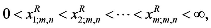
Suppose the experimenter provides a time T, which is an ideal total test time, but we may allow the experiment to run over time T. If the m-th progressively censored observed failure occurs before time T (i.e.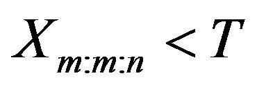 ), the experiment stops at the time
  (see Figure 1). Otherwise, once the experimental time passes time T but the number of observed failures has not reached m, we would want to terminate the experiment as soon as possible.
This setting can be viewed as a design in which we are assured of getting m observed failure times for efficiency of statistical inference and at the same time the total test time will not be too far away from the ideal time T. From the basic properties of order statistics (see, for example, David and Nagaraja [10]), we know that the fewer operating items are withdrawn (i.e., the larger the number of items on the test), the smaller the expected total test time (Ng and Chan [11]). Therefore, if we want to terminate the experiment as soon as possible for fixed value of m, then we should leave as many surviving items on the test as possible. Suppose J is the number of failures observed before time T, i.e.

where  and
and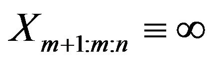 . According to the above result on stochastic ordering of first order statistics

Figure 1. Experiment terminates before time T (i.e. xm:m:n < T).
from different sample sizes, after the experiment passed time T, we set 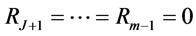 and
and
 . This formulation leads us to terminate the experiment as soon as possible if the
  -th failure time is greater than T for
 . Figure 2 gives the schematic representation of this situation. The value of T plays an important role in the determination of the values of
  and also as a compromise between a shorter experimental time and a higher chance to observe extreme failures. One extreme case is when
 , which means time is not the main consideration for the experimenter, then we will have a usual progressive Type-II censoring scheme with the pre-fixed progressive censoring scheme
 . Another extreme case can occur when
 , which means we always want to end the experiment as soon as possible, then we will have
  and
and  which results in the conventional Type-II censoring scheme.
If the failure times of the n items originally on the test are from a continuous population with cdf  and pdf
  for
for  the likelihood function is given by (see Ng et al. [1])
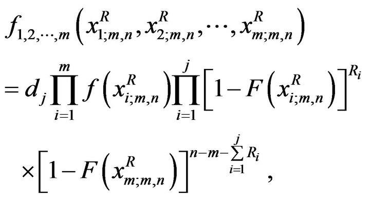 (3)
(3)
where
 (4)
(4)
3. Maximum Likelihood Estimation
Let 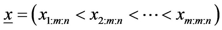 be an adaptive typeII progressive censored order statistics from generalized Pareto (GP) distribution, with censoring scheme
 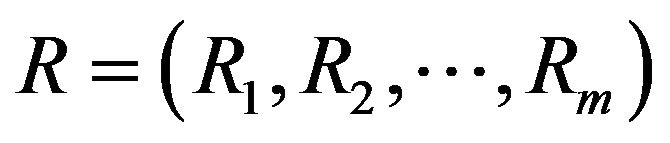 . From (1)-(3), the likelihood function is given by
 (5)
(5)
where  is defined in (4) and
  is used instead of
 .
.
The log-likelihood function may then be written as
 (6)
(6)
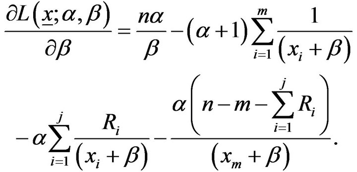
Upon differentiating (6) with respect to  and
and , and equating each result to zero, we get the likelihood equations as
 (7)
(7)
and
 (8)
(8)
hence from (7) we obtain the ML estimate of  as
as
 (9)
(9)
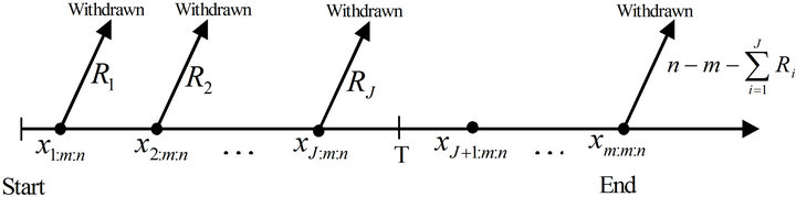
Figure 2. Experiment terminates after time T (i.e. xm:m:n ≥ T).
By using (9) in (8) we obtain
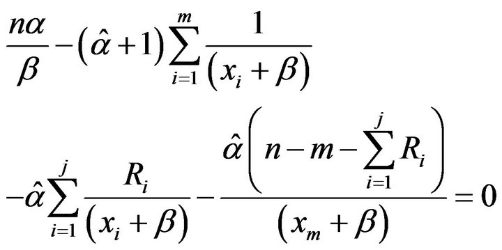 (10)
(10)
Since Equation (10) cannot be solved analytically for , some numerical methods such as Newton’s method must be employed to solve (10) and get the MLE
3.1. Approximate Interval Estimation
From the log-likelihood function in (6), we have
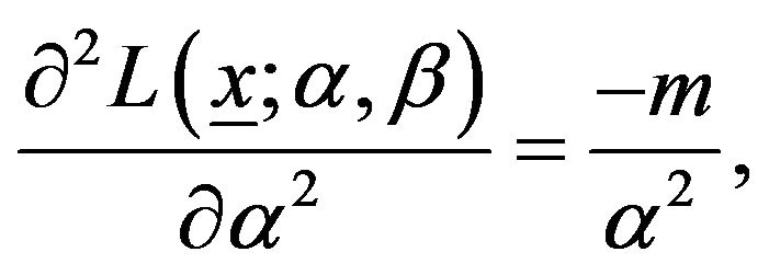 (11)
(11)
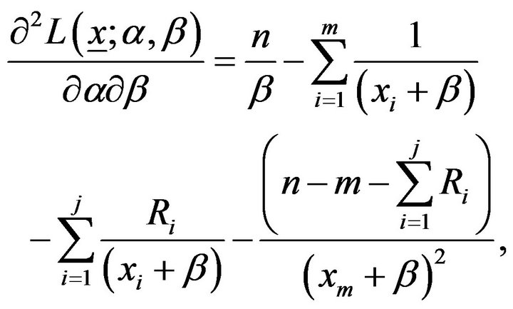 (12)
(12)
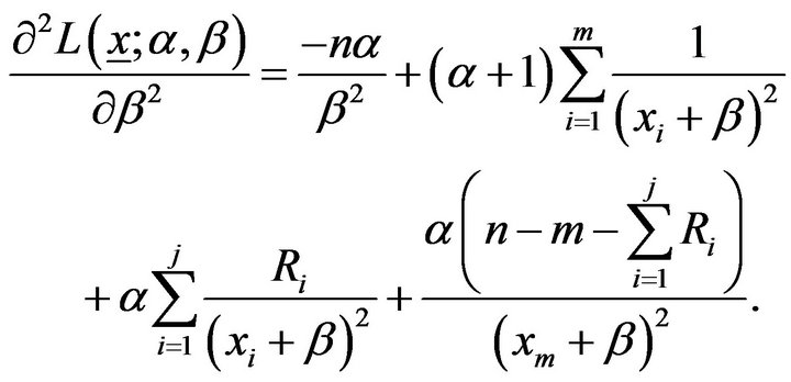 (13)
(13)
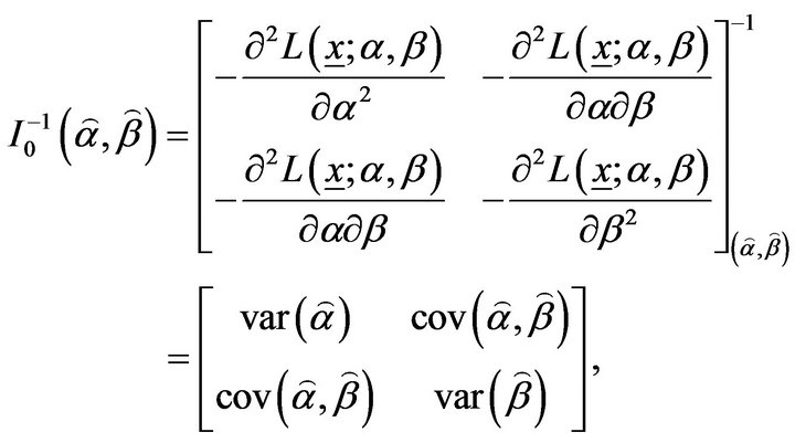
The Fisher information matrix  is then obtained by taking expectation of minus Equation (11)-(13). Under some mild regularity conditions,
  is approximately bivariately normal with mean
  and covariance matrix
 . In practice, we usually estimate
  by
by . A simpler and equally valued procedure is to use the approximation
where  is observed information matrix
approximate confidence intervals for  and
and  can be found by to be bivariately normal distributed with mean
  and covariance matrix
 . Thus, the
  approximate confidence intervals for
  and
and  are
are
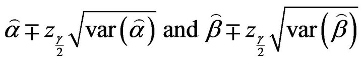 (14)
(14)
respectively, where  and
and  are the elements on the main diagonal of the covariance matrix
  and
and  is the percentile of the standard normal distribution with right-tail probability
 .
.
4. Bootstrap Confidence Intervals
In this section, we propose to use confidence intervals based on the parametric percentile bootstrap method (Boot-p) based on the idea of Efron [12]. The algorithms for estimating the confidence intervals of the parameters using (Boot-p) method is illustrated as the following1) From the original data
 compute the ML estimates of the parameters:
  and
and  from Equation (9) and solving the nonlinear Equation (10), respectively.
2) Use  and
and  to generate a bootstrap sample
  with the same values of
 ,
, ;
;  using algorithm presented in Ng et al. [1].
3) As in Step 1, based on  compute the bootstrap sample estimates of
  say
say .
.
4) Repeat Steps 2 - 3 N times representing N bootstrap MLE’s of  based on N bootstrap samples.
5) Arrange all ,
,  , in an ascending order to obtain the bootstrap sample
  Where
Where  Let
Let  be the cumulative distribution function of
 . Define
  for given
  The approximate bootstrap
  confidence interval of
  is given by
 (15)
(15)
5. Bayes Estimation and Credible Intervals
In this section we describe how to obtain the Bayes estimates and the corresponding credible intervals of parameters  and
and  when both are unknown. For computing the Bayes estimates, we assume mainly a squared error loss (SEL) function only; however, any other loss function can be easily incorporated.
In some situations where we do not have sufficient prior information, we can use non-informative prior distribution. This is particularly true for our study. For example, the non-informative uniform prior distribution can be used for parameters  and
and . The joint posterior density will then be in proportion to the likelihood function.
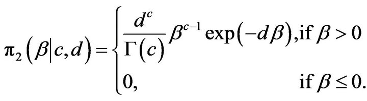
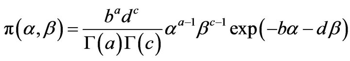
Here we consider the more important case when  is the shape parameter and
  is the scale parameter has independent gamma priors with the pdfs
 (16)
(16)
and
 (17)
(17)
Multiplying  by
by  we obtain the joint prior density of
  and
and ; given by
 (18)
(18)
Based on the likelihood function of the observed sample is same as (5) and the joint prior in (18), the joint posterior density of  and
and  given the data is
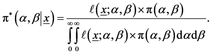 (19)
(19)
Therefore, the Bayes estimate of any function of  and
and  say
say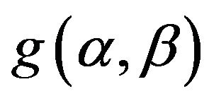 , under squared error loss function is
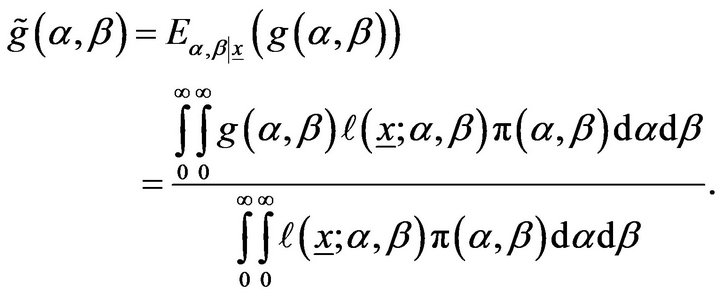 (20)
(20)
It is not possible to compute (20) analytically even when 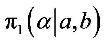 is known explicitly. Therefore, we propose the approaches of MCMC technique to approximate (20). See, for example, Robert and Casella [13] and Recently, Rezaei, et al. [14].
The MCMC method provides an alternative method for parameter estimation. It is more flexible when compared with the traditional methods. Moreover, probability intervals are available. The probability intervals provide us a reasonable interval estimate about the unknown parameter. In the following subsection, we propose using the MCMC technique to compute Bayes estimates of the unknown parameters and to construct the corresponding credible intervals.
5.1. The Metropolis-Hastings—Within-Gibbs Sampling
The Metropolis-Hastings algorithm is a very general MCMC method first developed by Metropolis, et al. [15] and later extended by Hastings [16]. It can be used to obtain random samples from any arbitrarily complicated target distribution of any dimension that is known up to a normalizing constant. In fact, Gibbs Sampler is a special case of a Monte Carlo Markov chain algorithm. It generates a sequence of samples from the full conditional probability distributions of two or more random variables. Gibbs sampling requires decomposing the joint posterior distribution into full conditional distributions for each parameter and then sampling from them. We propose using the Gibbs sampling procedure to generate a sample from the posterior density function 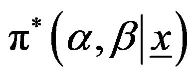 and in turn compute the Bayes estimates and also construct the corresponding credible intervals based on the generated posterior sample see Soliman, et al. [17,18]. In order to use the method of MCMC for estimating the parameters of the Lomax distribution, namely,
  and
and . Let us consider independent priors (16) and (17), respectively, for the parameters
  and
and . The joint posterior density function can be obtained up to proportionality by multiplying the likelihood with the prior and this can be written as
 (21)
(21)
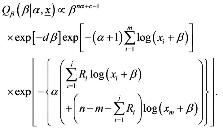
The posterior is obviously complicated and no closed form inferences appear possible. We, therefore, propose to consider MCMC methods, namely the Gibbs sampler, to simulate samples from the posterior so that samplebased inferences can be easily drawn. From (21), the posterior density function of  given
given  is proportional to
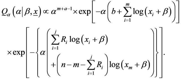 (22)
(22)
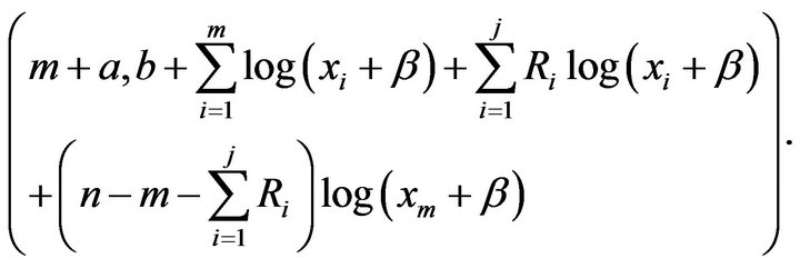
It can be seen that Equation (22) is a gamma density with shape parameter  and scale parameter
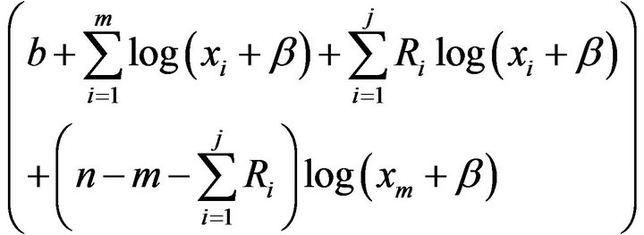
and, therefore, samples of  can be easily generated using any gamma generating routine. Similarly, the posterior density function of
  given
given  is proportional to
 (23)
(23)
The posterior density function of  given
given  Equation (23) cannot be reduced analytically to well known distributions and therefore it is not possible to sample directly by standard methods, but the plot of it shows that it is similar to normal distribution. So, to generate random numbers from this distribution, we use the Metropolis-Hastings method with normal proposal distribution.
Now, we propose the following scheme to generate  and
and  from the posterior density functions and in turn obtain the Bayes estimates and the corresponding credible intervals.
1) Start with an 
2) Set .
.
3) Generate  from Gamma
4) Using Metropolis-Hastings (see, Metropolis et al. [15]), generate  from
from  with the
  proposal distribution. Where
  is variances-covariance’s matrix.
5) Compute ,
,  .
.
6) Set 
7) Repeat steps 3-6  times.
8) Obtain the Bayes estimates of  and
and  with respect to the SEL function as
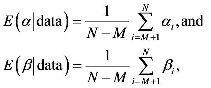
where M is burn-in.
9) To compute the credible intervals of  and
and , order
  and
and  as
as  and
and  Then the
  symmetric credible intervals of
  and
and  become

6. Illustrative Examples
To illustrate the inferential procedures developed in the preceding sections, we choose the real data set which was also used in Lawless (1982-pp 185). These data are from Nelson [19] concerning the data on time to breakdown of an insulating fluid between electrodes at a voltage of 34 k.v. (minutes). The 19 times to breakdown are
| 0.96 | 4.15 | 0.19 | 0.78 | 8.01 | 31.75 | 7.35 | 6.50 | 8.27 | 33.91 |
| 32.52 | 3.16 | 4.85 | 2.78 | 4.67 | 1.31 | 12.06 | 36.71 | 72.89 |
Example 1. In this case we take  and
and . Thus, the adaptive progressive censored sample is
Example 2. Now consider that  and
and  and
and ’s are same as before. In this case the adaptive progressive censored sample is
The point estimates of the parameters using the maximum likelihood (ML) method and Bootstrap (Boot-p) are presented in Table 1. Because we have no prior information about the unknown parameters, we assume the non-informative prior (prior 0: the joint posterior distribution of unknown parameters is proportional to the likelihood function). Based on the MCMC samples of size 10000 with 1000 as burn-in, the Bayes estimates of  and
and  are presented in Table 1. Also the 95% asymptotic, Boot-P confidence intervals and also the 95% credible intervals of
  and
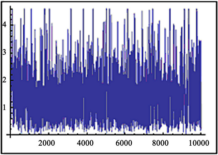
and  in Table 2. From these tables as expected the Bayes estimates under the non-informative prior and the MLE are quite close to each other. A trace plot is a plot of the iteration number against the value of the draw of the parameter at each iteration. Figure 3 displays 10000 chain values for the two parameters
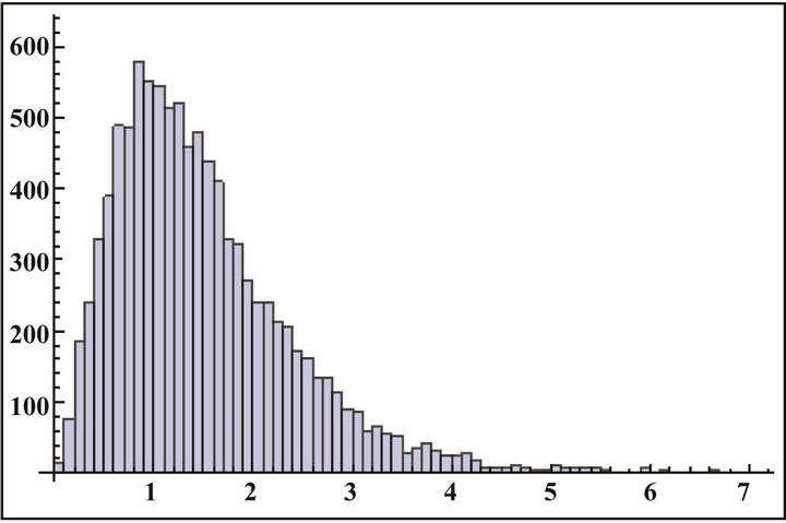
  and their histograms are shown in Figure 4 with these settings.
7. Monte Carlo Simulations
In order to compare the different estimators of the parameters, we simulated 1000 an adaptive Type-II progressive samples from Lomax distribution with the values of parameters  and different censoring schemes
 . The samples were simu
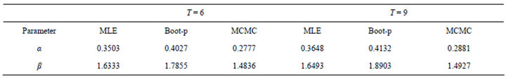
Table 1. The point estimates of MLE, Boot-p and MCMC of α and β.
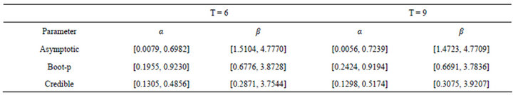
Table 2. 95% asymptotic, Boot-p and MCMC confidence (credible) intervals of α and β.
 (a)
(a) (b)
(b)
Figure 3. (a) (b) MCMC output of  and
and 
 (a)
(a)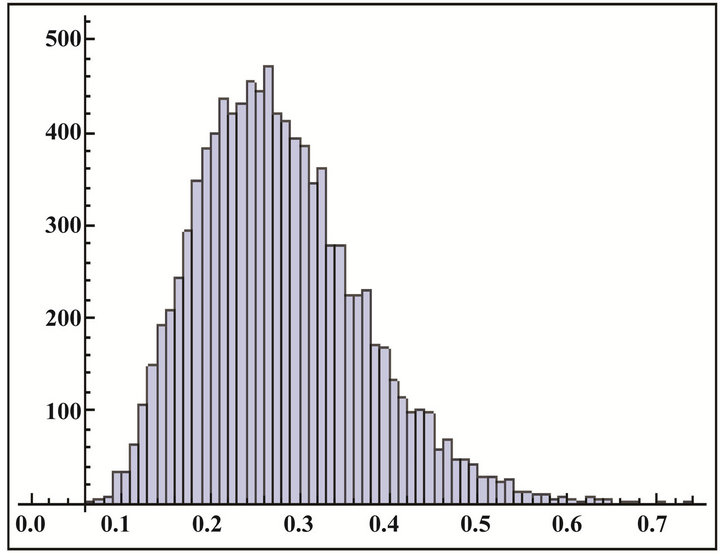 (b)
(b)
Figure 4. (a) (b) Histogram of  and
and 
lated by using the algorithm described in Ng, et al. [3]. We mainly compare the performances of ML and Bayes estimates with respect to the squared error loss function in terms of mean squared errors (MSEs). We also compare different confidence intervals, namely the confidence intervals obtained by using asymptotic distributions of the MLEs, bootstrap confidence intervals and the symmetric credible intervals in terms of the coverage percentages. All of the computations were performed by (mathematics 7.0) using a Pentium IV processor. To find the Bayes MCMC estimates, we used the noninformative gamma priors for the two parameters (we call it prior 0). Non-informative prior  provides prior distributions which are not proper, we also used an informative priors, including prior 1, a = 1, b = 2, c = 1, d = 2, with the values of previous parameters. We computed the Bayes estimates and
  probability intervals based on 10000 MCMC samples and discard the first 1000 values as burn-in. We report the mean squared errors (MSEs) and the coverage percentage (C.V) based on 1000 replications in Tables 3-6.
8. Conclusions
Recently Ng, et al. [3] suggest an adaptive Type-II progressive censoring. A properly planned adaptive progressively censored life testing experiment can save both the total test time and the cost induced by failure of the units and increase the efficiency of statistical analysis. In this article, we have considered the maximum likelihood (ML)and Bayes estimates for the parameters of the generalized Pareto (GP) distribution using adaptive Type-II progressive censoring scheme. Also, we develop different confidence intervals, namely the confidence intervals obtained by using asymptotic distributions of the MLEs, bootstrap confidence intervals and the symmetric credible intervals for the parameters of the generalized Pareto (GP) distribution. A simulation study was conducted to examine and compare the performance of the proposed methods for different sample sizes, and different censoring schemes.
From the results obtained in Tables 3-6, it can be seen that the performance of the MLEs is quite close to that of the Bayes estimators with respect to the noninformative priors, as expected. Thus, if we have no prior information on the unknown parameters, then it is always better to
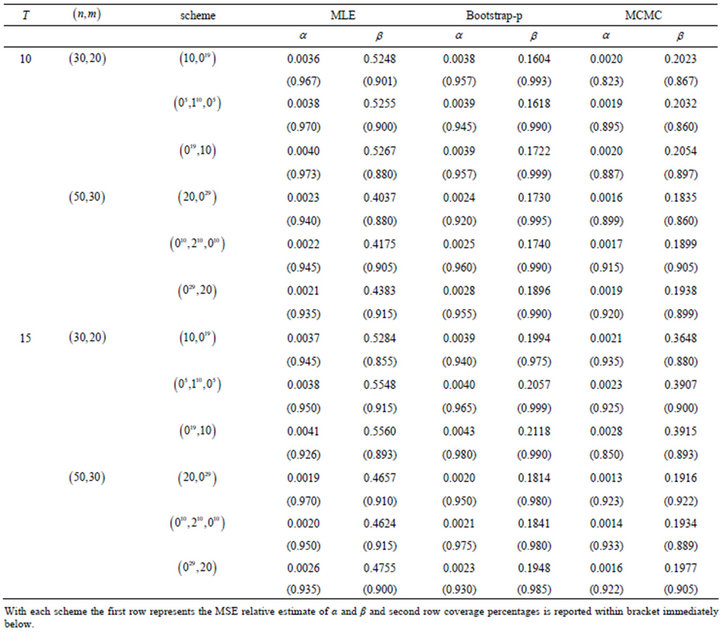
Table 3. Mean squared errors (MSEs) relative estimate of parameters and coverage percentages (C.V) with  and prior 0.
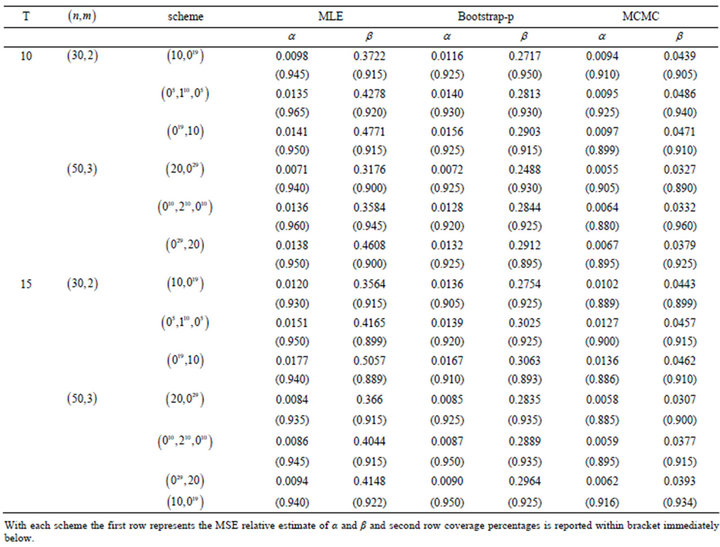
Table 4. Mean squared errors (MSEs) relative estimate of parameters and coverage percentages (C.V) with  and prior 1.

Table 5. The average confidence lengths relative estimate of parameters with 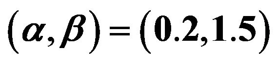 and prior 0.
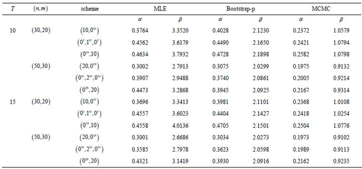
Table 6. The average confidence lengths relative estimate of parameters with  and prior 1.
use the MLEs rather than the Bayes estimators, because the Bayes estimators are computationally more expensive.
REFERENCES
- H. K. T. Ng, D. Kudu and P. S. Chan, “Statistical Analysis of Exponential Lifetimes under an Adaptive Type-II Progressive Censoring Scheme,” Naval Research Logistics, Vol. 56, No. 8, 2010, pp. 687-698. doi:10.1002/nav.20371
- N. Bal Krishnan, “Progressive Censoring Methodology: An Appraisal,” Test, Vol. 16, No. 2, 2007, pp. 211-296. doi:10.1007/s11749-007-0061-y
- N. Bal Krishnan and R. Aggarwala, “Progressive Censoring: Theory, Methods, and Applications,” Birkhauser, Boston, Berlin, 2000.
- K.S. Lomax, “Business Failure: Another Example of the Analysis of the Failure Data,” Journal of the American Statistical Association, Vol. 49, No. 268, 1954, pp. 847- 852. doi:10.1080/01621459.1954.10501239
- M. Habibullah and M. Ahsanullah, “Estimation of Parameters of a Pareto distribution by Generalized Order Statstics,” Communication in Statistics, Theory and Methods, Vol. 29, No. 7, 2000, pp. 1597-1609. doi:10.1080/03610920008832567
- S. K. Upadhyay and M. Peshwani, “Choice between Weibull and Lognormal Models: A Simulation Based Bayesian Study,” Communication in Statistics, Theory and Methods, Vol. 32, No. 2, 2003, pp. 381-405. doi:10.1081/STA-120018191
- A. H. Abd Ellah, “Bayesian One Sample Prediction Bounds for the Lomax Distribution,” Indian Journal Pure and Applied Mathematics, Vol. 34, No. 1, 2003, pp. 101- 109.
- A. H. Abd Ellah, “Comparison of Estimates Using Record Statstics from Lomax Model: Bayesian and Non Bayesian Approaches,” Journal of Statistical Research and Training Center, Vol. 3, No. 2, 2006, pp. 139-158.
- E. Cramer and G. Iliopoulos, “Adaptive Progressive Type-II Censoring,” Test, Vol. 19, No. 2, 2010, pp. 342- 358. doi:10.1007/s11749-009-0167-5
- H. A. David and H. N. Nagaraja, “Order Statistics,” 3rd Edition, Wiley, New York, 2003. doi:10.1002/0471722162
- H. K. T. Ng and P. S. Chan, “Comments on Progressive Censoring Methodology: An Appraisal,” Test, Vol. 16, No. 2, 2007, pp. 287-289. doi:10.1007/s11749-007-0071-9
- B. Efron, “The Jackknife, the Bootstrap and Other Resampling Plans,” CBMS-NSF Regional Conference Seriesin, Applied Mathematics, SIAM, Philadelphia, Vol. 38, 1982.
- C. P. Robert and G. Casella, “Monte Carlo Statistical Methods,” 2nd Edition, Springer, New York, 2004. doi:10.1007/978-1-4757-4145-2
- S. Rezaei, R. Tahmasbi and M. Mahmoodi, “Estimation of P[Y
- N. Metropolis, A. W. Rosenbluth, M. N. Rosenbluth, A. H. Teller and E. Teller, “Equations of State Calculations by fast Computing Machines,” Journal Chemical Physics, Vol. 21, No. 6, 1953, pp. 1087-1091. doi:10.1063/1.1699114
- W. K. Hastings, “Monte Carlo Sampling Methods Using Markov Chains and Their Applications,” Biometrika, Vol. 57, No. 1, 1970, pp. 97-109. doi:10.1093/biomet/57.1.97
- A. A. Soliman, A. H. Abd-Ellah, N. A. Abou-Elheggag and E. A. Ahmed, “Reliability Estimation in StressStrength Models: An MCMC Approach,” Statistics, 2011, pp. 1-14.doi:10.1080/02331888.2011.637629
- A. A. Soliman, A. H. Abd-Ellah, N. A. Abou-Elheggag and E. A. Ahmed, “Modified Weibull Model: A Bayes Study Using MCMC Approach Based on Progressive Censoring Data,” Reliability Engineering and System Safety, Vol. 100, No. 2, 2012, pp. 48-57. doi:10.1016/j.ress.2011.12.013
- W. B. Nelson, “Applied Life Data Analysis,” Wiley, New York, 1982. doi:10.1002/0471725234
NOTES
*Mathematics Subject Classification: 62N05; 62F10.