Intelligent Information Management
Vol.2 No.8(2010), Article ID:2499,10 pages DOI:10.4236/iim.2010.28055
Semi-Markovian Model of Monotonous System Maintenance with Regard to Operating Time to Failure of Each Element
Sevastopol National Technical University, Sevastopol, Ukraine
E-mail: vmsevntu@mail.ru
Received May 12, 2010; revised June 18, 2010; accepted July 21, 2010
Keywords: Maintenance, Semi-Markovian Process, System Stationary Characteristics, System Performance Indexes Optimization
Abstract
An explicit form of reliability and economical stationary performance indexes for monotonous multicomponent system with regard to its elements’ maintenance has been found. The maintenance strategy investigated supposes preventive maintenance execution for elements that has attained certain operating time to failure. Herewith for the time period of elements’ maintenance or restoration operable elements are not deactivated. The problems of maintenance execution frequency optimization have been solved. For the model building the theory of semi-Markovian processes with a common phase field of states is used.
1. Introduction
In the process of a complex engineering system opera-tion its components’ characteristics are deteriorating. One of the methods of system stationary performance indexes improvement is the preventive maintenance of its components. From a large number of monographs and scientific papers dealing with mathematical aspects of systems’ maintenance the works [1-8] should be singled out. Among other subjects, the single-component system maintenance strategy known as “Depending-on-age restoration” [2] or “The rule of preventive replacement” [1,5] is investigated in them. The essence of this strategy is the following. The system is restored after its failure. If it has been operating without failures for the given time period , its maintenance is carried out. For this strategy the rates of operation expenses and the availability function have been found, the problem of definition of maintenance execution optimal periodicity has been solved. In the present paper this maintenance strategy is generalized for multicomponent systems with monotonous structure [2]. The examples of the systems with mo-notonous structure are serial, parallel, parallel-serial, serial-parallel, and bridge ones.
The goal of the present article is to define optimal values of monotonous multicomponent system’s components operating time for the maintenance execution with the purpose of gaining best stationary reliability and economical characteristics of the system.
2. The Problem Definition and Mathematical Model Building
Let us consider N-component system with a monotonous structure [2]. Such systems as serial, parallel, bridge systems, “P of N” systems, the ones with the whole-seg-regated redundancy fall into category of the system investigated.
The failure-free operation time of system’s i-element is a random value (RV)  with distribution function (DF)
  . The failure indication of element is carried out instantly and its emergency restoration (ER) which lasts random period of time
  with DF
  begins. If system’s i-ele-ment has been operating without failures for the given time period
  , then its maintenance, the duration of which is RV
  with DF
 is to be executed. It is assumed that all the RV are independent and have an absolutely continuous DF and finite assembly averages
  There is no restoration queue. Both after maintenance and after ER all the reliability characteristics of elements are completely restored. The operating time to failure level
  for system’s i-element maintenance is determined both after maintenance and after ER. Elements’ deactivation and activation in the system are carried out instantly. The income per time unit of system’s good state, expenses per time unit of emergency restoration and of system’s i-element maintenance are equal respectively
  and
and 
The system is in up state only then when at least one of the serial structures of minimal path [2] is also in up state. The system is considered to be in down state when at least one of the parallel structures of minimal section [2] is in down state (owing to its elements’ maintenance or ER). It is assumed that neither ER nor maintenance of any element results in deactivation of the operable elements that are functionally connected with the failed component and do not belong to any other up-state path.
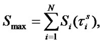
The task is to determine the following system’s per-formance indexes: stationary steady state availability factor  , mean specific income
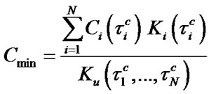
  per calendar time unit, and mean specific expenses
  per time unit of system’s good state. It is also necessary to determine the values of elements’ operating time
  . On attaining these values elements’ maintenance should be executed to optimize the above-mentioned system performance indexes.
Time diagram of system operation is shown in Figure 1.
Let us describe the system operation by means of se-mi-Markovian process  with discretely continuous phase field of states [9,10]
where the components of vector  indicate
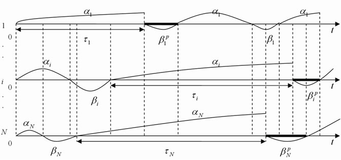
Figure 1. Time diagram of multicomponent system operation without deactivation of elements with regard to their maintenance in age.
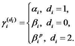
physical state of elements:  – k points out that kelement is in up state,
  indicates ER state of it,
  signifies its maintenance state; i is the number of element, which was last to change its physical state. The components of vector
  record time period between the moment of i-element’s last state change and the nearest moments of the rest of elements’ state change respectively
  . If
. If  then
then  is time till the next emergency failure of k-element. The components of vector
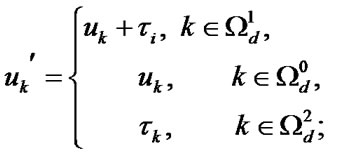
 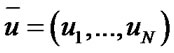 are equal to the values of respective elements’ operating time from the moment of their ER or maintenance. If
  then it is considered that
  . At the moment of i-element’s up state restoration after its maintenance or ER its operating time is equal to zero:
  .
.
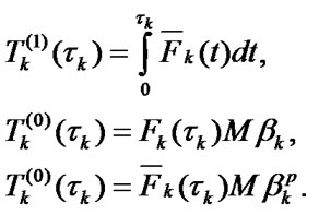
Time periods of system’s dwelling in its states are defined by ratios:
 where
where  is a sign of minimum;
  is a set of numbers of vector
  components that are equal to 1,
Let us describe the probabilities (probability densities) of embedded Markovian chain (EMC)  transition. It is necessary to note that i-element can change its physical state 1 into the state 0 (ER) and into the state 2 (maintenance) but the states 0 and 2 can be changed only into the state 1.
Let us indicate 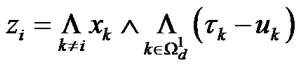 and let
  ,
,  be sets of numbers of vector
  components that are equal to 0 and 2, respectively. The state
  admits the following transitions:
1) to the set of states  with the probability density of transition
 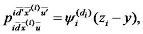 where
where  is the density of probability distribution of RV
  ,
,
2) to the set of states 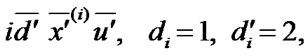 with transition probability
 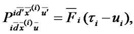 where
where 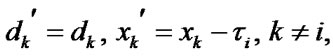
3) to the set of states 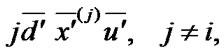 with the probability density of transition
 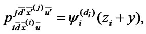 where
where

Let us assume that the conditions of stationary distribution [9,10] existence and uniqueness for EMC  are fulfilled. The following theorem takes place.
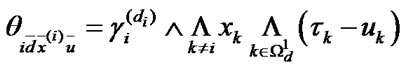
Theorem. The stationary distribution  of EMC
  is defined by the following expressions: as the Equation (1).
One can check this statement validity by the direct substitution of expression (1) to the set of integral equa-tions, determining the stationary distribution of EMC.
3. Definition of System Stationary Characteristics
Let us divide the phase field  of system states into two non-overlapping subsets
  and
and  ;
;  is a subset of up states,
  is a subset of down states:
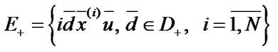 ,
,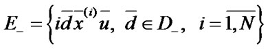 .
.
Here  is a set of vectors
  the components of which are equal to the codes of physical states of (down) states
  One should note that element’s maintenance is referred to the down states.
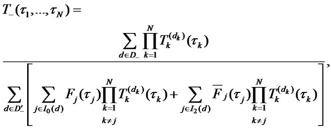
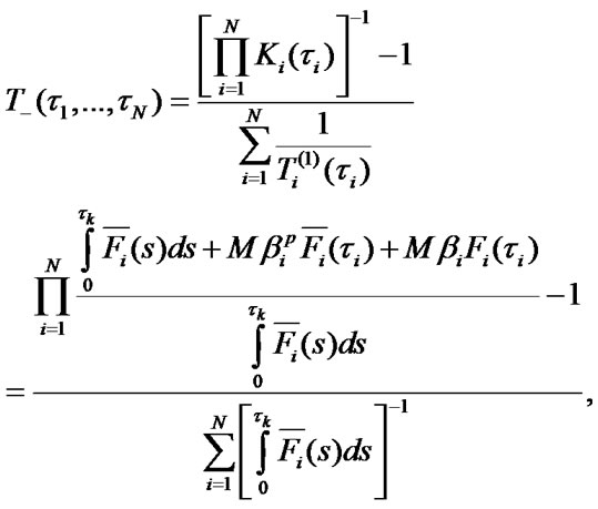
Mean stationary operating time to failure  , mean stationary restoration time
  , and stationary steady state availability factor (SSAF)
  will be defined with the help of formulas [9,10]
 (1)
(1)
 (2)
(2)
where  is the stationary distribution of EMC
  ,
,  are mean time periods of system’s dwelling in its states,
 are pro-babilities of EMC
  transition from down (up) states to up (down) states.
With regard to the stationary distribution of EMC (1) the Formula (2) is transformed into:
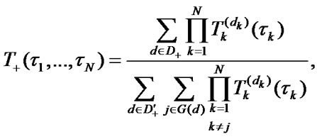 (3)
(3)
 (4)
(4)
 (5)
(5)
Here  is a set of system’s borderline physical up states, that is a set of such vectors
  that any component change from 1 to 0 or to 2 transfers vector
  to the set
  ;
;  is a set of such numbers of vector
  components that any component change from 1 to 0 or to 2 transforms vector
  to the set
  ;
;  is a set of system’s borderline down states, that is a set of such vectors
  that any component change from 0 or 2 to 1 transforms vector
  to the set
  ;
;  is a set of such numbers of vector
  components that any component change from 0 (2) to 1 transforms vector
  to the set
  .
.
Remark. If passive strategy of elements’ maintenance is executed, i.e., elements’ maintenance is not carried out, then the Formulas (3)-(5) coincide with respective stationary characteristics of restorable systems [9,10]. It becomes clear when taking into account that:
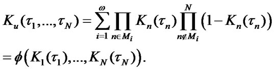
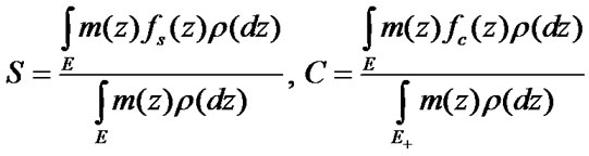
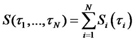
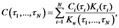
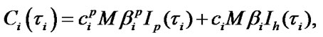
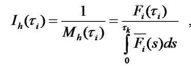
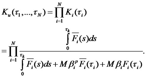
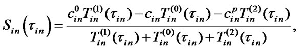
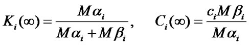
Let us define system stationary characteristics 
 using SSAF
  of elements that are defined by Formulas [1,2]:
Let  be all the different sets of elements of system paths [2]. One should note that according to the definition the elements not belonging to the set of elements of path is in down state, i.e., are in a state 0 or 2.
  are the sets of borderline paths elements;
  is a set of borderline path
  elements that correspond to the numbers of elements, the transition of which from up to down state, leads to the whole system failure. The sets
  are the ones of section elements;
  are the sets of borderline section elements;
  is a set of borderline section
  elements that correspond to the numbers of the elements, the transition of which from down to up state leads to the whole system restoration.
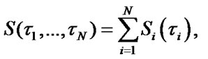
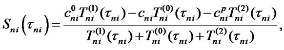
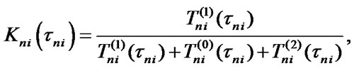
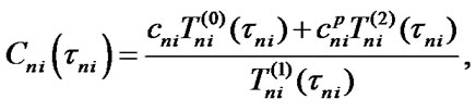
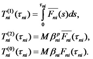
Formulas (3)-(5) transformation of averages products’ sums and some other elementary transformations lead to the following result:
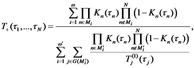 (6)
(6)
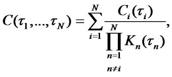
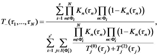 (7)
(7)
 (8)
(8)
Here the structural function of the system  is given in a disjunctive normal form but it can be introduced in many different equivalent forms, for example, in a linear one [2,11].
To define mean specific income  per calendar time unit and mean specific expenses
  per time unit of system’s good state, the formulas [12] will be used
 (9)
(9)
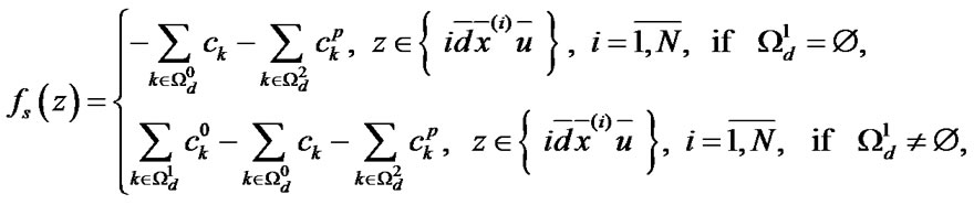
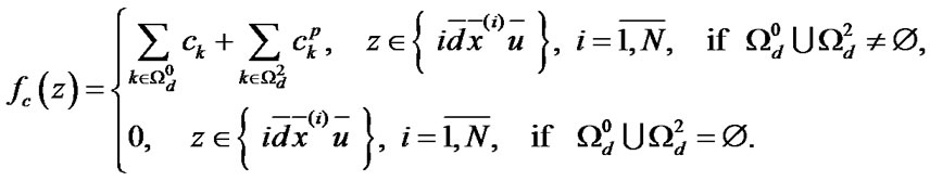
where  ,
,  are the functions defining income and expenses respectively in every state.
With regard to indications introduced in the model building part of the article the functions  and
and  gain the bottom form:
After some transformations the Formula (9) will be as following:
 ,
,
 (10)
(10)
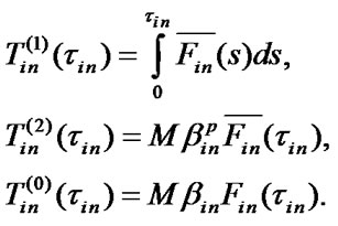
where 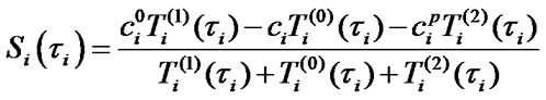 is mean specific income of i-element per calendar time unit and
 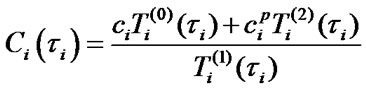 are mean specific expenses per time unit of i-element’s good state. One should note that in [2] the value of mean specific expenses
  is called “operating expenses rate” and is presented in the following form:
where 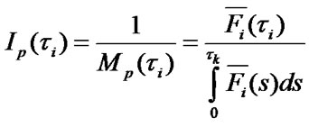
 are respectively an average number of ER and maintenance per time unit;
 are assembly averages of time period between ER and maintenance of i-element.
Hereafter let us write down stationary characteristics of multicomponent systems with concrete structures and with regard to their elements’ maintenance in age.
Stationary characteristics of serial system. The block scheme of N-component serial system is shown in Figure 2.
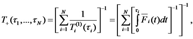
Let us use the ratios (6)-(8). The system has a single borderline path:  Emergency failure of any element or its maintenance leads to the whole system failure, that is why
  The structural function of the system
  is the following one:
 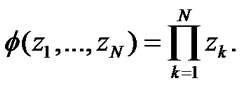 Thus, mean stationary
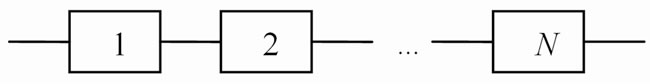
Figure 2. Block scheme of serial system.
|
|
operating time to failure , mean stationary restoration time
  and stationary steady state availability factor of the system
  are defined by the following expressions:
The system mean specific income per calendar time unit and mean specific expenses per time unit of sys-tem’s good state are estimated with the help of ratios:
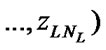
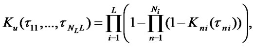
Stationary characteritics of parallel system. In Figure 3 the block scheme of N-component redundant system of integer multiplicity with active reserve is shown.
The system has a single borderline section: 

 In this case the structural function of the system
  will be
 According to the Formulas (6)-(8), (10) system stationary performance indexes are defined by the equations:


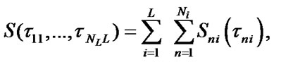
Stationary characteristics of parallel-serial system. The block scheme of parallel-serial system is shown in Figure 4.
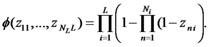
It includes L serial chains with parallel connection. Each i-chain consists of  elements in series. In this instance the structural function of the system
 is as follows:
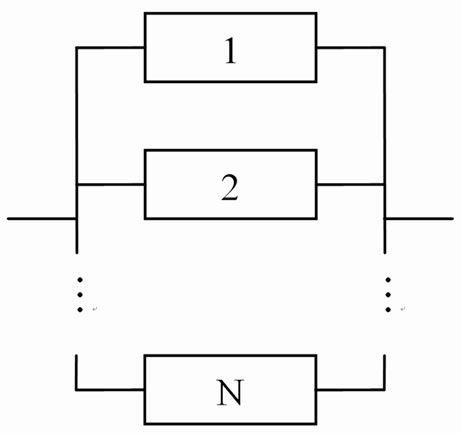
Figure 3. Block scheme of parallel system.
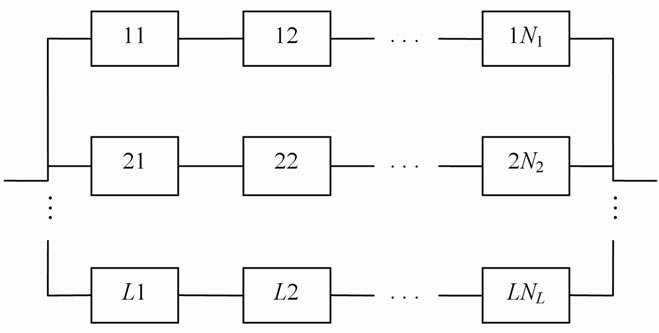
Figure 4. Block scheme of parallel-serial system.
 The ratios (8), (10) for stationary characteristics estimation of this structure are transformed into the following expressions:
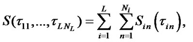
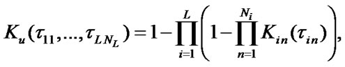
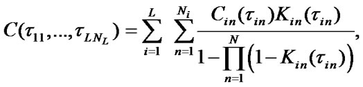
where  are stationary SSAF, mean specific income of i-chain’s
  -element per calendar time unit and mean specific expenses per time unit of this element’s good state respectively:


Stationary characteristics of serial-parallel system. In Figure 5 the block scheme of serial-parallel system is represented.
It consists of L units in series. Each i-unit includes  parallel elements. In this case the structural function of the system
  is
is
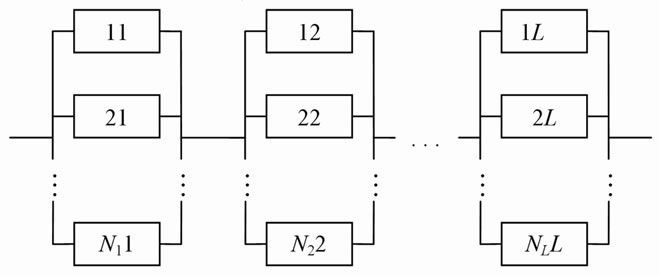
Figure 5. Block scheme of serial-parallel system.
 According to (8), (10) system stationary characteristics can be estimated in the following way:
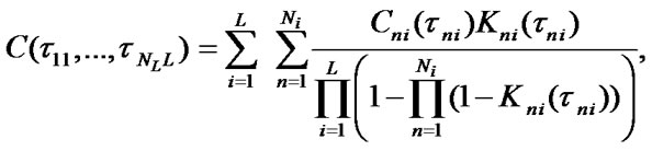
where 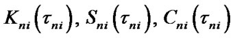 are stationary SSAF, mean specific income of i-unit’s
  -element per calendar time unit and mean specific expenses per time unit of this element’s good state respectively:
4. Optimization of Elements Maintenance Terms
The task of defining optimal system’s performance indexes is reduced to the definition of absolute extremums of the functions (8) and (10). It is necessary to note that for gaining maximum values of system SSAF
 and mean specific income
 it is obligatory and sufficient to optimize the value of each system element’s operation time for its maintenance execution, which is not valid for system’s minimum mean specific expenses
 .
.
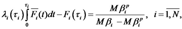
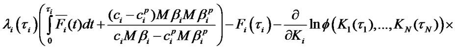
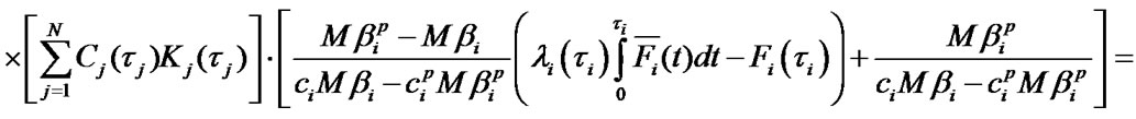
Equaling the partial derivatives of the functions  and
and  to zero we get the systems of equations defining optimal values of operating time
 :
:
 (11)
(11)
as the Equations (12) and (13)
Here 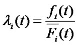 is the continuous failure rate of
  -element.
The sufficient condition for the systems of Equations (11), (13) finite solutions existence is respective inequalities fulfillment (it is supposed that  for the system (13)).
In case of systems of equations’ unique solutions existence, optimal values of system performance indexes are defined by the following formulas:
 ,
,
 , (14)
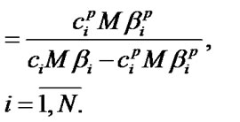
 , (12)
 (13)
(13)
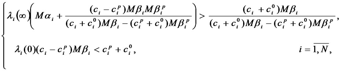


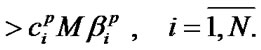
Table 1. System initial data.
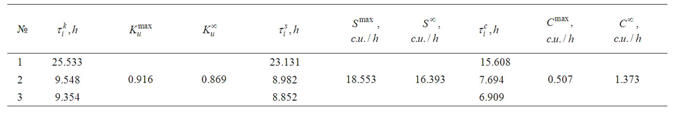
Table 2. Calculation results.
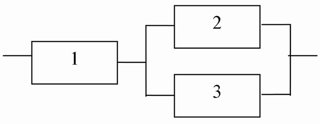
Figure 6. System block scheme for an example.
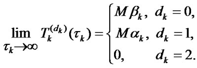
If the systems of equations have several solutions, optimal values of system performance indexes are found by substituting each one to the formula for the case of unique solution with subsequent choice of the best variant. The absence of roots of any  -equation of the systems (11), (12) denotes that the function
 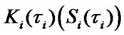 is a monotone one and its extremum is attained under
 . In this case it should be assumed that
 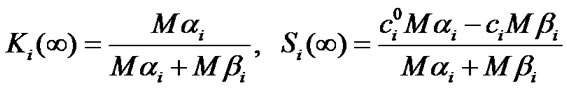 in the Formula (14).
If the system of Equation (13) doesn’t have any solutions, all the possible functions that result from (10) after the substitution of
should be analyzed for absolute minimum. Extremum attainment under  signifies that it is not expedient to execute
  -element’s maintenance because it deteriorates system performance indexes.
In conclusion an example of optimal maintenance exe-cution terms definition for three-component system with the structure represented in Figure 6 will be given. Its elements’ operating time to failure is disposed according to the law of Veibull-Gnedenko with densities:
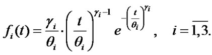
Initial data and calculation results are represented in the Tables 1 and 2.
Here  denote system performance in-dexes in case if elements’ maintenance is not carried out. The elements’ maintenance execution increases these indexes for 5.406%, 13.178%, 63.068% respectively.
5. Conclusions
In the present paper semi-Markovian model of operation of multicomponent restorable system with monotonous structure, which takes into account its elements’ main-tenance execution depending on the values of operating time to failure, has been built. With the help of this model the reliability and economical stationary chara-cteristics of the system with a general form of elements’ time to failure and restoration time distributions have been defined. These characteristics are explicitly depen-dent on the periodicity of system of system elements’ maintenance execution. This fact allows solving the pro-blems of the above-mentioned characteristics’ improve-ment. For a single-component system the quality indexes found coincide with the formerly known ones [1,2]. In case when elements’ maintenance is not carried out ( ), the stationary indexes coincide with the ones found in [9,10] for restorable systems. In prospect the analogical model of maintenance of multicomponent system operating under the condition of elements’ deactivation will be built by the authors.
6. References
[1] R. E. Barlow and F. Proschan, “Mathematical Theory of Reliability,” John Wiley and Sons, New York, 1965.
[2] F. Baichelt and P. Franken, “Reliability and Maintenance: A Mathematical Approach,” Radio and Communication, Moscow, 1988.
[3] Y. Y. Barzilovich and V. A. Kashtanov “Some Mathe-matical Aspects of Complex Systems’ Maintenance Theory,” Soviet Radio, Moscow,1967.
[4] I. B. Gertsbakh, “Models of Preventive Maintenance,” North Holland Publishing Company, Amsterdam, New York, 1977.
[5] R. E. Barlow and L. Hunter, “Optimum Preventive Maintenance Policies,” Operations Research, Vol. 8, No. 1, 1960, pp. 90-100.
[6] C. Valdez-Flores and R. M. Feldman, “A Survey of Preventive Maintenance Models for Stochastically Deteriorating Single-Unit Systems,” Naval Research Logistics, Vol. 36, No. 4, 1989, pp. 419-446.
[7] D. I. Cho and M. Parlar, “A Survey of Maintenance Models for Multi-Unit Systems,” European Journal of Operational Research, Vol. 51, No. 2, 1991, pp. 1-23.
[8] R. Dekker and R. A. Wildeman, “A Review of Multi-Component Maintenance Models with Economic De-pendence,” Mathematical Methods of Operations Resear-ch, Vol. 45, No. 3, 1997, pp. 411-435.
[9] V. S. Korolyuk and A. F. Turbin, “Markovian Restoration Processes in the Problems of System Reliability,” Naukova dumka, Kiev, 1982.
[10] A. N. Korlat, V. N. Kuznetsov, M. I. Novikov and A. F. Turbin, “Semi-Markovian Models of Restorable and Service Systems,” Kishinev, Shtiintsa, 1991.
[11] A. M. Polovko and S. V. Gurov, “Bases of Reliability Theory,” Saint Petersburg, 2006.
[12] V. M. Shurenkov, “Ergodic Markovian Processes,” Nauka, Moscow, 1989.