Intelligent Information Management
Vol.2 No.9(2010), Article ID:2779,14 pages DOI:10.4236/iim.2010.29061
Optimal Task Placement of a Serial Robot Manipulator for Manipulability and Mechanical Power Optimization
1School of Mechanical Engineering, Federal University of Uberlândia, Uberlândia, Brazil
2Faculty of Mathematics, Federal University of Uberlândia, Uberlândia, Brazil
E-mail: rsantos9@gmail.com, vsteffen@mecanica.ufu.br, saramago@ufu.br
Received January 1, 2010; revised May 19, 2010; accepted July 20, 2010
Keywords: Optimal task placement, Optimal robot path planning, Multicriteria optimization
Abstract
Power consumption and accuracy are main aspects to be taken into account in the movement executed by high performance robots. The first aspect is important from the economical point of view, while the second is requested to satisfy technical specifications. Aiming at increasing the robot performance, a strategy that maximizes the manipulator accuracy and minimizes the mechanical power consumption is considered in this work. The end-effector is constrained to follow a predefined path during the optimal task positioning. The proposed strategy defines a relation between mechanical power and manipulability as a key element of the manipulator analysis, establishing a performance index for a rigid body transformation. This transformation is used to compute the optimal task positioning through the optimization of a multicriteria objective function. Numerical simulations regarding a serial robot manipulator demonstrate the viability of the proposed methodology.
1. Introduction
Minimization of production costs and maximization of productivity are some of the major objectives of industrial automation. In this scenario, serial robot manipulators have been proved to be very useful tools.
Due to the augmenting use of serial robot manipulators to perform a number of tasks in industry, requirements concerning higher precision, improved productivity, reduced costs, and better manufacturing quality become very important. To effectively explore all the potential of the robot, its path planning is a subject of major concern.
There are several works in the literature dedicated to different approaches concerning this subject. Regarding the off-line path planning approach, in Saramago [1] a solution of moving a robot manipulator with minimum cost along a specified geometric path in the presence of moving obstacles is presented. The optimal traveling time and the minimum mechanical energy of the actuators are considered together to form a multiobjective function to be minimized along the process.
In Santos [2] a strategy to determine the trajectory for a defined movement taking into account the requirements of torque, velocity, operation time and robot positioning along the movement is proposed. The analysis is performed as an off-line path planning through spline interpolation techniques in the manipulator joint space. In the paper of Chiddarwar [3] an off-line path planning for coordinated manipulation is proposed. The swept sphere volume technique is used to model multiple robots and static obstacles. In Santos [4] the trajectory of two manipulators while manipulating a single object in a collaborative task and the object placement are written as an optimization problem. End-effector positioning and torque requirements are considered together in an optimal control formulation. Accuracy and energy consumption are improved during the path planning. Also, the flexibility effects of manipulators working in a vertical workspace are taken into account, and joint limits are considered in a box-constrained objective function to ensure the movement feasibility at the optimal configuration.
In von Stryk [5] an optimal control path-planning strategy for which the dynamics of the robot and the total traveling time are considered as objectives to be optimized is proposed. In Santos [6] an optimal control strategy that considers the presence of moving obstacles in the workspace is presented.
The problem of time-optimal control along a specified path has been investigated for several authors (Bobrow [7], Slotine [8]). In Constantinescu [9] a smooth timeoptimal strategy for serial robot manipulators is presented.
The paper of Seraji [10] addressed a geometric approach to determine the appropriate base location from which a robot can reach a target point. The work of Zeghloul [11] presented some kinematic performance criteria for the optimal placement of robots, and proposed a general optimization method to determine the placement of manipulators automatically.
In Feddema [12], an algorithm for determining the optimal placement of a robotic manipulator for minimum time coordinated motion is proposed. In Park [13] a study that characterizes a set of desired goal positions and a left-invariant distance metric parametrized by length scale is studied.
The paper of Chirikjian [14] proposed several metrics to be used to generate interpolated sequences of motions of a solid body. In Martinez [15] an analysis regarding the metric of a rigid displacement obtained from the kinematic mapping is presented and other metrics for the set of spatial and planar displacements are proposed. The work of Tabarah [16] proposed an optimization strategy for determining the optimal base for a given manipulator, and two cooperating manipulators, following a continuous path with constant velocity. They considered the constant velocity as a constraint. A strategy for velocity minimization is proposed by Zhang [17], based on a neural network solver. A kinematic planning scheme is reformulated as a quadratic problem that is solved by using a real-time algorithm, and applied to a Puma 560 robotic arm.
In Abdel-Malek [18] a strategy regarding the placement of a robot manipulator aiming at reaching a specified set of target points is described. The placement of a serial manipulator in a given workspace is achieved by defining the position and orientation of the manipulator’s base with respect to a fixed reference frame. The strategy is based on characterizing the robot placement by adjusting a constrained cost function that represents the workspace to a set of target points.
With the aim of increasing productivity in the path following, industrial robotic applications have been addressed in the literature by determining path-constrained time-optimal motions, by taking into account the torque limits of the actuators. In these formulations, the joint actuator torques are considered as controlled inputs and the open loop control schemes result in bang-bang or bang-singular-bang controls (Bobrow [7], Chen [19], Shiller [20]). The paper of Xidias [21] proposed the generalization of the task scheduling problem for articulated robots in a constrained 2D environment. An algorithm for the optimum collision-free movement is proposed.
However, the increase of the speed may result (in some cases) in increasing the robot end-effector vibration or decreasing its accuracy. This is observed due to several factors, such as the bang-bang nature of the control, joint flexibility, joint friction, gear arrangement, or even a combination of them.
Vibration is not desired because it can both degrade the system performance and decrease the actuator lifetime. A related and negative effect of vibration is the poor accuracy of the system.
The present contribution discusses an alternative way to improve the overall performance of serial robot manipulators. The use of manipulability and mechanical power related indexes to achieve the best task placement is proposed.
As the basic idea of manipulability consists in describing directions in the task or joint space that maximizes the ratio between some measure of effort in joint space and a measure of performance in task space, the present contribution consists in the optimal positioning of the task to be performed, which results in the maximization of the robot manipulability and the minimization of the required mechanical power. This will lead to accuracy maximization and power consumption minimization, since manipulability can be understood as an ability measurement (Fu [22]) and mechanical power is related to power consumption (Saramago [1]).
In the present paper both kinematics and dynamics features are considered in the proposed task placement strategy. From the best of the authors’ knowledge, this problem was not previously addressed in the literature, despite its importance and applicability.
The position of the end-effector is fixed according to a Cartesian reference system, and described as a sequence of sucessive positions. The optimization process applies a translational and rotational transformation matrix with respect to a given reference frame. As a result, an optimal sequence of kinematical robot positions is determined.
The outline of the paper is the following. In Section 2, a review about manipulability is presented. In Section 3, the mechanical power concept is discussed. A strategy to describe the task and its positioning in the design space is proposed in Section 4. Additionally in this section the design variables are defined. In Section 5 the multicriteria programming formulation is presented. In Section 6, the optimization strategy is established and the numerical experiments are performed in Section 7. Finally, the conclusions are drawn in Section 8.
2. Manipulability
Some factors should be taken into account when the posture of the manipulator in the workspace is determined for performing a given task during operation. An important factor is the ease of arbitrarily changing the position and orientation of the end-effector at the tip of the manipulator.
As an approach for evaluating quantitatively the ability of manipulators from the viewpoint of kinematics, the concepts of manipulability ellipsoid and manipulability measure (Yoshikawa [23]) are presented.
Consider a manipulator with n degrees of freedom. The joint variables are denoted by an n-dimensional vector, q = [q1, q2, ..., qn]T. An m-dimensional vector r = [r1, r2, ..., rm]T, (m ≤ n) describes the position and orientation of the end-effector.
The relation between the velocity vector v corresponding to r and the joint velocity  is given by:
 (1)
(1)
where J(q) is the Jacobian matrix, computed from the kinematics description of the robot.
The set of all end-effector velocities v that are realizable by joint velocities such that the Euclidean norm of  satisfies
  defines an ellipsoid in the m-dimensional Euclidean space. In the direction of the major axis of the ellipsoid, the end-effector can move at high speed, and in the direction of the minor axis, the end-effector can move only at low speed. Also, the larger the ellipsoid is, the faster the end-effector can move.
Since this ellipsoid represents an ability of manipulation, it is called the manipulability ellipsoid.
The principal axes of the ellipsoid can be found by making use of the singular-value decomposition of J(q).
One of the representative measures for the ability of manipulation derived from the manipulability ellipsoid is the volume of the ellipsoid. Since this volume is proportional to the eigenvalues of the Jacobian, it can be seen as a representative measure. Therefore, the manipulability measure, f1, for the manipulator configuration, q, is defined as
 (2)
(2)
Generally f1 ≥ 0 holds, and f1 = 0 if and only if rank J(q) < m.
There is a direct relation between singular configuration and manipulability (through the Jacobian concept). According to this relationship, it can be shown that the larger the manipulability measure, the larger the ability of avoiding singular configurations.
3. Mechanical Power
The consideration of the dynamics behavior of a serial robot manipulator is of great importance for its path planning. This information allows a detailed analysis and consequently the development of a precise control specification.
Many efficient schemes have been proposed to model the dynamics of rigid multibody mechanical systems (Richard [24], Mata [25], Mata [26]). The dynamics model can be obtained explicitly through algebraically computation, or numerically through iterative computation.
The techniques based on the Newton-Euler method starts from the dynamics of all individual parts of the system. They look at the instantaneous or infinitesimal aspects of the motion, using vector quantities such as Cartesian velocities and forces.
Alternatively, the Euler-Lagrange based methods starts from the kinetic and potential energy of the entire system, by considering the states of the system during a finite time interval. This approach works with scalar quantities, namely the energies.
Independently of the approach used, at the end of the process the generalized forces are determined:
 (3)
(3)
where  and
and  are the joint position, velocity and acceleration, respectively. M(q) is the joint space mass matrix and
  is the vector of Coriolis and centrifugal forces. Vector g(q) is the vector of gravitational forces and τ is the generalized force vector.
The energy that is necessary to move the robot is an important design issue, because in real applications energy supply is limited and any energy reduction leads to smaller operational costs. Due to the relationship that exists between energy and force, the minimal energy can be estimated from the generalized force,  , that is associated to each joint i at the time instant t0 ≥ t ≥ tf.
In the present contribution, for a manipulator with n degrees of freedom, the interval between the initial time t0 and the final time tf is represented by a set of N points and the computation is numerically carried out through a recursive Newton-Euler formulation (Craig [27]). Then, the mechanical power is used for design purposes as defined by:
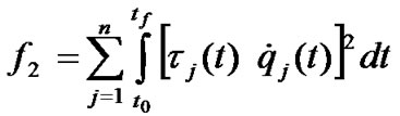 (4)
(4)
This expression is representative of the phenomenon under study because it considers both the kinematics and the dynamic aspects of the trajectory, simultaneously (Saramago [1]).
4. Task Specification
The task is specified as a set S of N Cartesian points (x, y, z) and the respective time step. Hence,
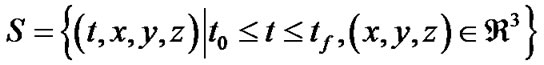 . (5)
. (5)
In the case of non-redundant manipulators there exist a finite number of configurations that satisfies the end-effector positioning specification. This path-following problem is a highly constrained task, and the inverse kinematics problem will have four solutions or less.
Considering the need of movement continuity together with a time-fixed specification at each step and a relative small step size, the point-to-point path planning strategy may fail due to the complexity of the constraints.
Therefore, a task positioning optimization is proposed as an alternative to increase the robot performance without changing the position of the task reference points with respect to each other. In other words, all the points will be moved simultaneously through a rigid body transformation to find the best position from the point of view of the ability of the manipulator.
To achieve this goal, the use of a homogeneous transformation A is proposed, which in this case is defined as
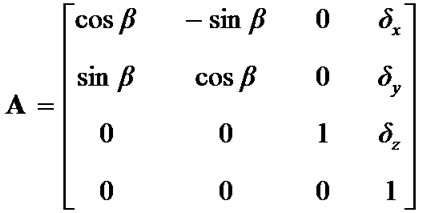 (6)
(6)
where β is a rotation angle in the z axis (given in rad) and δx , δy and δz are translations along the reference axes (given in meters), respectively. If desired, it is possible to extend this formulation to consider the rotation with respect to the reference axes.
The physical meaning of considering a rotation angle with respect to x or y is that the robot’s base plane will not be parallel to the ground’s reference plane. In other words, the robot’s z axis (its height) is not normal to the ground’s reference plane (xy plane). As positioning two planes according to a precise angle may not be possible in a number of practical situations (even when it is possible, it is not an easy procedure to be done, in general terms), the rotation along the z axis only is considered, maintaining the robot’s base plane parallel to the task’s base plane.
After defining the set S that describes the task, the inverse kinematics with respect to each Cartesian point is computed.
The inverse kinematics computation can be achieved algebraically, by considering the analytical model of the manipulator and its geometry, or numerically. With the aim of presenting a general procedure, in the present contribution the inverse kinematics problem is solved numerically through an inverse problem formulation. This approach results an efficient and general procedure that works satisfactorily for manipulators exhibiting arbitrary complexity (Santos [28]).
The obtained path planning presents an end-effector positioning error, while the robot executes the path. The interest is focused on errors due to task positioning, as the inverse kinematics can generally be solved with a sufficient precision.
Once the objective is specified, it is necessary to define the optimization domain, i.e., the design space. As the design variables are defined in a theoretical space (defining a rigid body transformation) and the positioning constraints are defined in the Cartesian space (the workspace), a constraint parameter is included in the formulation.
Defining the theoretical positioning error at each point as
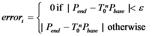 (7)
(7)
where Pbase, Pend and  are the robot base point, the end-effector point, and the kinematics representation of the manipulator, respectively. The penalty parameter used as a constraint in the following optimization formulation is given by
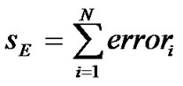 (8)
(8)
and represents the sum of all end-effector positioning errors during the movement.
Equation (7) means that the end-effector error is considered null when the accuracy is better than the one specified by ε (given in meters). Otherwise, this error corresponds to the distance from the end-effector specified position to the position obtained from the direct kinematics calculation.
In some robotic implementations it is necessary to plan the layout of the workspace, i.e., it is required to locate the robot base in such a way that dexterity is maximized at (or around) given targets. It is worth mentioning that such cases are also covered by the present formulation. Since the optimal design ((β, δx, δy, δz) in Equation (6)) means a coordinate transformation of the end-effector path regarding the fixed robot base, it is also possible to adjust the location of the robot base regarding the fixed end-effector reference through the relation (-β, -δx, -δy, -δz).
5. Multicriteria Programming
In problems with multiple criteria, one deals with a design variable vector x, which satisfies all constraints and makes the scalar performance index that is calculated from the m components of an objective function vector f(x) as small as possible. This goal can be achieved by the vector optimization problem:
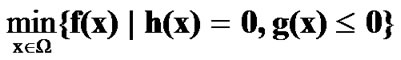 (9)
(9)
where Ω
 is the function domain (the design space).
An important feature of such multiple criteria optimization problem is that the optimizer has to deal with objective conflicts (Eschenauer [29]). Other authors discuss the same topic by defining compromise programming, because there is no unique solution to the problem (Vanderplaats [30]).
5.1. The Proposed Formulation
To consider together the manipulability and the total mechanical power, the following scalar objective function is proposed
 (10)
(10)
where f1 and f2 are given by Equations (2) and (4), respectively. The reference values  and
and  are obtained from the computation of the manipulability and mechanical power sum at the initial task positioning. Therefore, in the ideal case the objective function value is lower than 2, where
  (the manipulability was increased) and
  (the mechanical power was decreased).
The specification of a reference value to both the manipulability measure and the mechanical power are of paramount importance in the construction of the multicriteria objective function.
The inverse kinematics error is included in the problem as an equality constraint in the optimization formulation, through the expression sE = 0 (Equation (8)).
It should be pointed out that the proposed formulation is able to handle the case in which the task is outside the robot workspace. This configuration reflects in the inverse kinematics error, which is taken into account as a constraint (Equation (8)) of the optimization formulation.
Additionally, initial and final velocity specifications are considered as
 (11)
(11)
 (12)
(12)
for each joint j in the initial and final times t0 and tf, respectively. To represent a rest-to-rest motion, zero initial and final velocities are considered above.
6. Optimization Strategy
An important feature of the proposed analysis is the computation of highly nonlinear equations. Despite the good performance of classical nonlinear programming techniques, the global optimal design is hardly reached due to the existence of local minima in the design space.
With the aim of improving the robustness of the optimization process, the use of a global methodology is considered. The tunneling algorithm (Levy [31,32]) is a heuristic methodology designed to find the global minimum of a function. It is composed of a sequence of cycles, each cycle consists of two phases: a minimization phase having the purpose of lowering the current function value, and a tunneling phase that is devoted to finding a new initial point (other than the last minimum found) for the next minimization phase. This algorithm was first introduced by Levy [31], and the name derives from its graphic interpretation.
In summary, the computation evolves according to the following phases:
a) Minimization phase: Given an initial point q0, the optimization procedure computes a local minimum q* of f(q). At the end, it is considered that a local minimum is found.
b) Tunneling phase: Given q* found above, since it is a local minimum, there exists at least one q0 , such that
 (13)
(13)
In other words, there exists q0  Z = {q
  Ω – {q*} | f(q) ≤ f(q*) }. To move from q* to q0 along the tunneling phase, it is defined a new initial point q = q* + δ, q
  Ω that is used in the auxiliary function
 (14)
(14)
which has a pole in q* , for a sufficient large value of η By computing both phases iteratively, the sequence of local minima may lead to the desired global minimum..
Different values for η are suggested for being used in Equation (14) to avoid undesirable points and prevent the search algorithm to fail (Levy [31,32]). In the present case the stop criterion is five consecutive iterations without further improvement in the minimal objective value.
The minimization phase is performed by using a constrained formulation, where the objective function is given by Equation (10) and the constraint function is defined by Equation (8). The velocity specification (Equations (11) and (12)) is achieved through the determination of a suitable interpolation polynomial function using the joint position coordinates.
In Equation (14), during the tunneling phase, only the unconstrained formulation given by Equation (10) is considered. This unconstrained nonlinear programming problem is solved by using the BFGS variable metric method (Luenberger [33], Vanderplaats [30]). The constrained formulation of the minimization phase (Equations (10), (11) and (12)) is solved by using the modified method of the feasible directions (Vanderplaats [34]).
The algorithms are implemented in FORTRAN by using the optimization library DOT (Vanderplaats [35]).
7. Numerical Simulations
The numerical simulations performed to illustrate the presented methodology use two robot models, namely the Scara and the Puma 560 robot manipulators. These two types of serial robot manipulators are classical configurations in the field. The case studies have been proposed due to their complexity as compared to those normally found in the literature. The following results considers only optimal profiles whose sum of the end-effector error is zero (Equation (8)), given ε = 0.001 m (Equation (7)). This means that the inverse kinematics solution is found for all positions with the required precision. Different tolerance values may result from different optimal profiles.
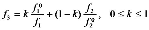
As different values for the weighting factor k lead to different optimization problems (Equation (10)), the value of the global minimum is normalized according to the following equation
 (15)
(15)
This performance index enables comparing the improvement of each objective without the weighting effect, and is used in the subsequent analysis.
In summary, the global optimization for each weighting factor (k = 0, 0.1, 0.2, 0.3, ..., 1) is performed according to Equation (10) and the comparison among the optimal designs obtained is performed by using Equation (15). Thus, eleven global optimizations for each task have been carried out. The maximum inverse kinematics error was defined as being lower than ε = 0.001 m in Equation (7).
A Scara manipulator was used in the first and second numerical experiments. The third numerical experiment refers to a Puma 560 manipulator. By considering the ability of describing a complex path, the data for a set of Cartesian specification points (Equation (5)) is determined through a cubic spline interpolation of the parametric coordinates of the desired path. Therefore, all the values are obtained from a suited set of Cartesian points.
The path for each experiment is arbitrarily defined with the aim of exploring the efficiency of the methodology in performing a complex task. All the obtained results consider only configurations for which inverse kinematics errors are lower than ε, i.e., sE = 0 (Equation (8)).
Each value k in Equation (10) defines a new optimization problem. To compare the values given by different optimization formulations, the normalization of the results, despite the weighting factor, is taken into account as established by f4 (Equation (15)).
7.1. First Experiment
In this experiment, a subset of 7 reference points is defined: (0, 0.4, 0, –0.3), (1, 0.4, –0.1, –0.3), (2, 0.2, –0.1, –0.3), (3, 0.2, –0.2, –0.3), (4, 0.4, –0.25, –0.3), (5, 0.4, –0.2, –0.3) and (6, 0.2, –0.25, –0.3). Comparing these values with Equation (5), the initial task is inside a rectangle defined by 0.2 ≤ x ≤ 0.4, –0.3 ≤ y ≤ –0.1 and z = –0.3. The corresponding traveling time is defined by 0 ≤ t ≤ 6. These data are computed by interpolating cubic splines for t, x, y and z, respectively. The interpolated data encompass a set of N = 27 points (Equation (5)) that describes the path-following problem, as presented in Figure 1.
At the original position, the values of the design variables are: β= 0 rad, δx = 0 m, δy = 0 m, and δz = 0 m. These values are used as an initial guess for the optimization process (Equation (10)).
The global minimum values obtained are presented in Figure 2.
The optimal values of manipulability and mechanical power indexes demonstrate that there is no clear dependence between the variables. Good results are provided for k = 0.2, 0.5, 0.6, and 0.9.
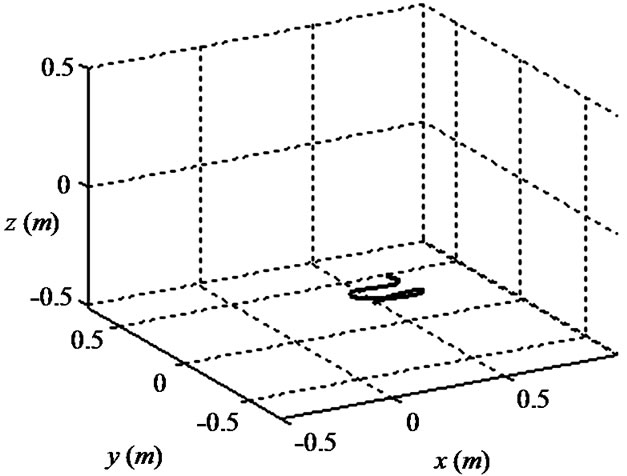
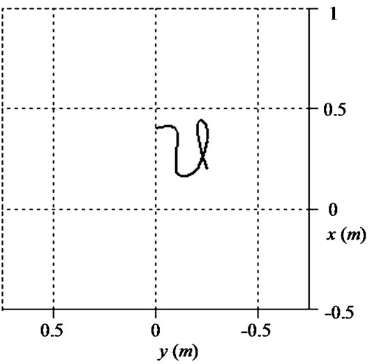
Figure 1. The proposed path-following problem from two different perspectives.
Details about the minimal performance index, k = 0.9, are presented in Table 1. The overall performance was improved 28%, while the minimal manipulability and the mechanical power were improved 62% and 18%, respectively.
Some of the values provided by other weighting factors may result in further improvement of the manipulability or mechanical power, separately. However, the present configuration is a global minimum of the performance index f4.
The improvement obtained during the tunneling process is shown in Figure 3.
After the 6th iteration of the tunneling process, no further improvement was achieved during the next five consecutive iterations. This behavior defines the stop criteria for the global optimization search. The above result highlights the good performance of the method, as satisfactory results are obtained after a small number of iterations.
Figure 4 shows the robot performing the path following task and Figure 5 presents the robot optimal positioning, according to the optimal design variable values
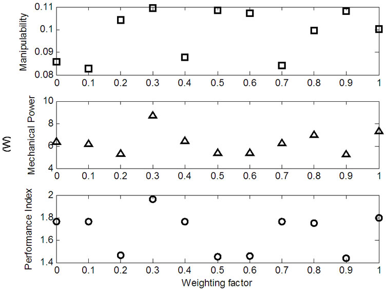
Figure 2. Optimal values obtained by using different weighting factors.
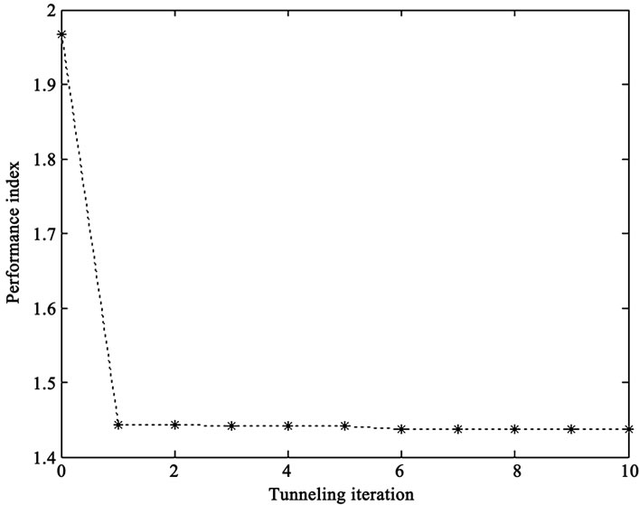
Figure 3. Performance index along the tunneling iterations (for k = 0.9).
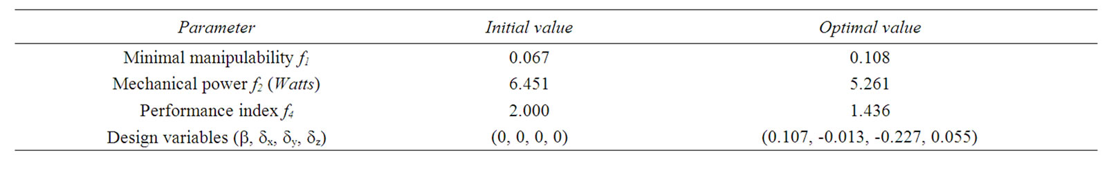
Table 1. Initial and optimal parameter values (for k = 0.9).
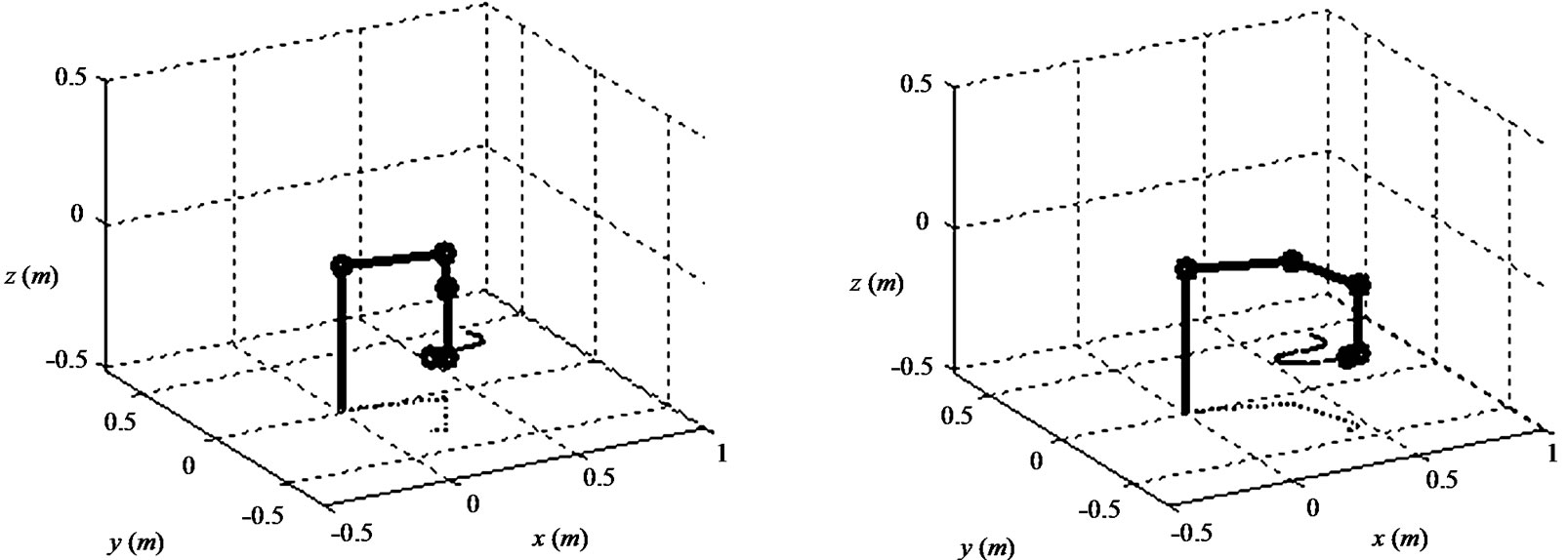
Figure 4. Robot performing the path following task.
given in Table 1.
The joint coordinates at each time step are obtained from inverse kinematics computation. Once the task is considered as a set of consecutive Cartesian points with continuous transition between them, the corresponding joint coordinates presents a smooth behavior. Figure 6 shows the initial and optimal joint coordinates of the first three links and the corresponding manipulability index.
Once the inverse kinematics is iteratively computed for each end-effector positioning, it is possible to include the obstacle avoidance feature in the above strategy. The corresponding procedure for the inverse kinematics computation is addressed in Santos [28], for example.
7.2. Second Experiment
In this experiment a subset of 8 reference points is defined: (0, 0.2, 0, –0.3), (1, 0.4, –0.1, –0.3), (2, 0.4, –0.05, –0.3), (3, 0.2, –0.1, –0.3), (4, 0.25, –0.15, –0.3), (5, 0.3, –0.17, –0.3), (6, 0.27, –0.13, –0.3) and (7, 0.26, –0.2, –0.3). By comparing these values with Equation (10), the initial task is inside a rectangle defined by 0.2 ≤ x ≤ 0.4, –0.2 ≤ y ≤ 0 and z = –0.3. The corresponding traveling time is defined by 0 ≤ t ≤ 7. These data are computed by interpolating cubic splines for t, x, y and z, respectively. The interpolated data encompass a set of N = 54 points
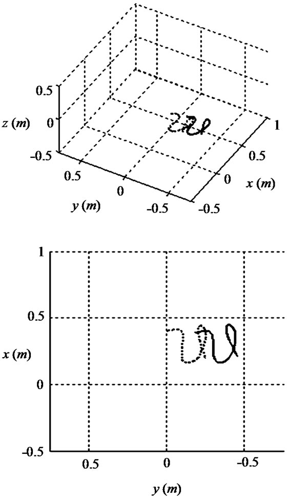
Figure 5. Proposed (---) and optimal (––) paths from two different perspectives.
(Equation (5)) that describes the path-following problem, as presented in Figure 7" target="_self"> Figure 7.
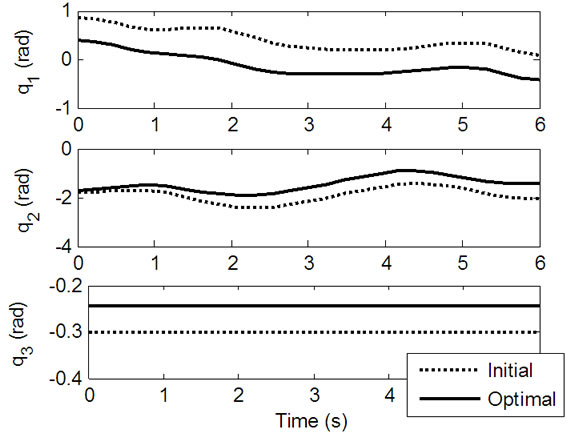
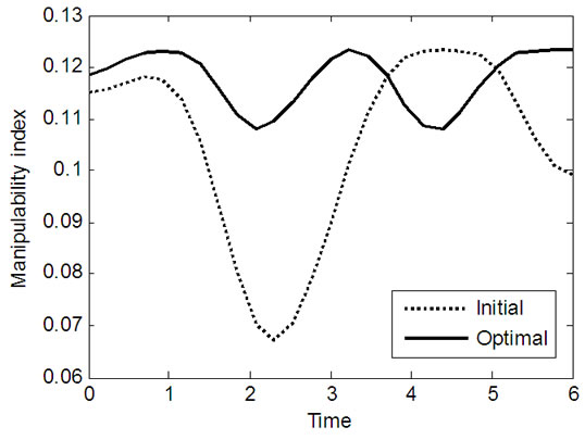
Figure 6. Joint coordinates and the corresponding manipulability index (Scara manipulator).
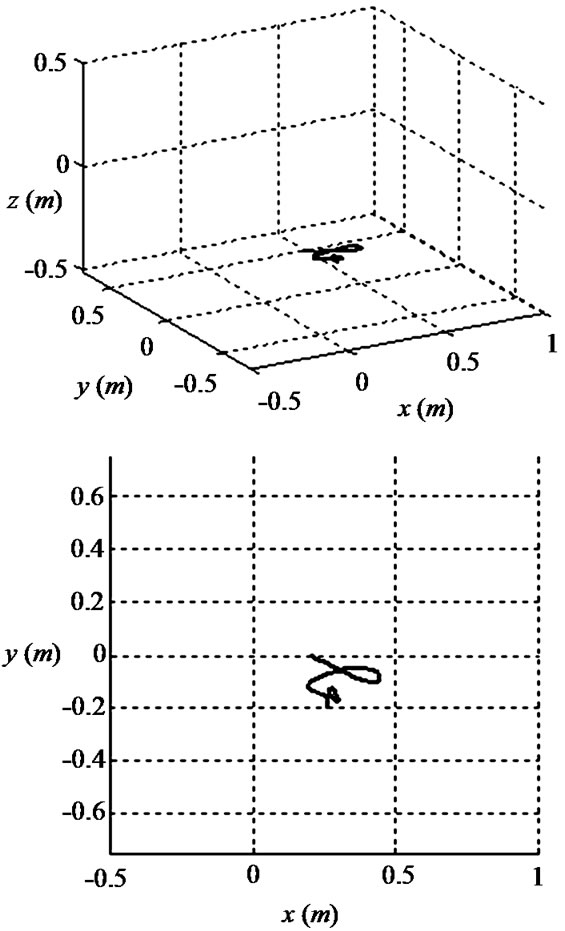
Figure 7. The proposed path-following problem from two different perspectives.
At the original position, the values of the design variables are: β = 0 rad, δx = 0 m, δy = 0 m, and δz = 0 m. These values are used as an initial guess for the optimization process (Equation (10)). Global optimizations were performed for eleven different values of the weighting factor k, (k = 0, 0.1, 0.2, ..., 1) (see Equation (10)).
The minimum values obtained by the optimization process are presented in Figure 8" target="_self"> Figure 8.
In this experiment good results are provided by k = 0.3, 0.4, and 0.7. Details about the minimal performance index, k = 0.7, are presented in Table 2. The overall performance was improved 17%, while the minimal manipulability and the mechanical power were improved 46% and 3%, respectively.
Eventually, the values provided by other weighting factors may result in further improvement either of the manipulability or the mechanical power, separately. However, the above configuration is a global minimum of the performance index f4.
The design improvement achieved by the tunneling process is shown in Figure 9" target="_self"> Figure 9.
After iteration 18 of the tunneling process, no further improvement was achieved for five consecutive iterations, defining the stop criterion of the global optimization search.
Figure 10 shows the robot performing the path-following task and Figure 11 presents the optimal positioning, according to the optimal design values presented inTable 2.
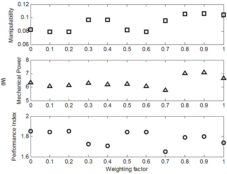
Figure 8. Optimal values obtained by using different weighting factors.
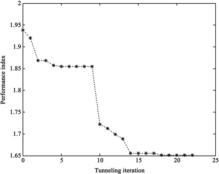
Figure 9. Performance index along the tunneling iterations (for k = 0.7).
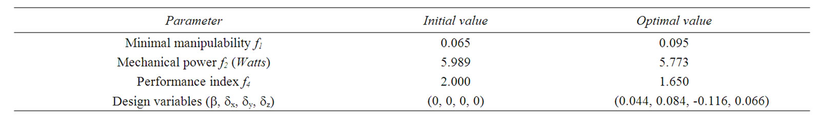
Table 2. Initial and optimal parameter values (for k = 0.7).
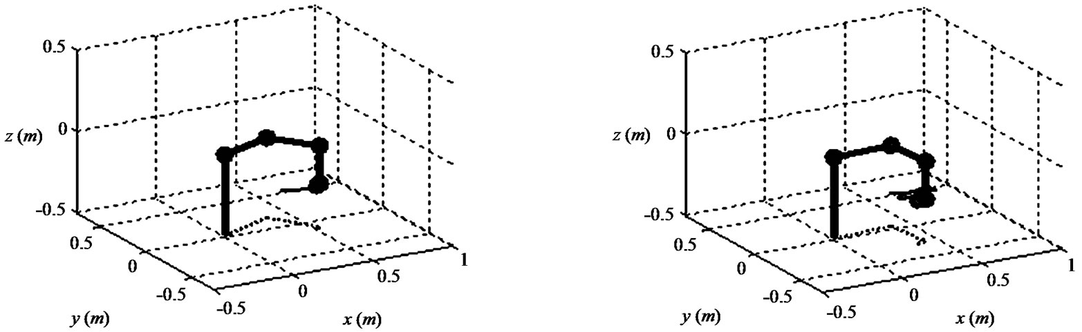
Figure 10. Robot performing the path-following task.
The joint coordinates at each time step are obtained by inverse kinematics computation. As the discrete set of points defining the task (Equation (5)) is supposed to describe a continuous path, the transition between joint coordinates is computed through cubic spline interpolation. Figure 12 shows the initial and optimal joint coordinates for the first three links and the corresponding manipulability index.
For the examples presented above, the task was defined as being parallel to the xy plane, i.e., the path is parallel to the ground.
7.3. Third Experiment
In this experiment, a subset of 7 reference points is defined: (0, 0.4, 0.1, 0), (1, 0.4, 0, 0), (2, 0.4, 0, –0.4), (3, 0.4, –0.3, –0.4), (4, 0.4, –0.4, 0), (5, 0.4, –0.3, 0), and (6, 0.4, –0.4, –0.4). By comparing these values with Equation (5), the initial task is inside a rectangle defined by x = 0.4, –0.4 ≤ y ≤ 0.1, and –0.4 ≤ z ≤ 0. The corresponding traveling time is defined by 0 ≤ t ≤ 6. These data are computed by interpolating cubic splines for t, x, y and z, respectively. The interpolated data encompass a set of N = 54 points (Equation (5)) that describe the path-following problem, as presented in Figure 13.
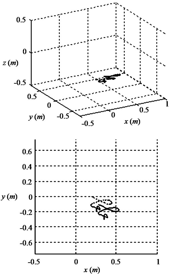
Figure 11. Proposed (---) and optimal (––) paths from two different perspectives.
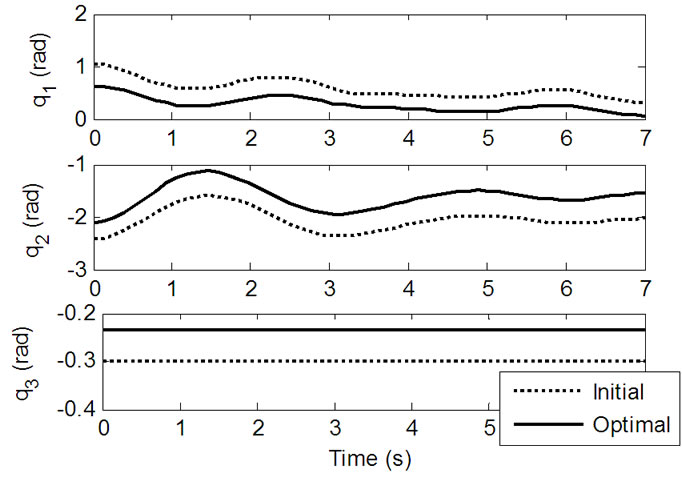
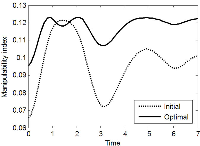
Figure 12. Joint coordinates and the corresponding manipulability index (Scara manipulator).
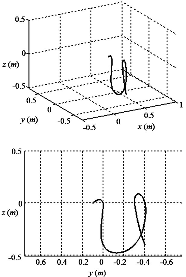
Figure 13. The proposed path-following problem from two different perspectives.
At the original position, the values of the design variables are: β = 0 rad, δx = 0 m, δy = 0 m, and δz = 0 m. These values are used as an initial guess for the optimization process (Equation (10)).
The optimal values of both the manipulability and the mechanical power indexes demonstrate that there is no significant difference among most of the results presented. The best values are provided by k = 0.4 and 0.5.
Details about the minimal performance index, k = 0.5, are presented in Table 3" target="_self"> Table 3. The overall performance was improved 40%, while the minimal manipulability and the mechanical power were improved 64% and 41%, respectively.
Some of the values obtained by using other weighting factors may result in further improvement of either the manipulability or the mechanical power, separately. However, the above configuration is a global minimum of the performance index f4.
The performance provided by the tunneling process is shown in Figure 14.
After the 5th iteration of the Tunneling process, no further improvement was achieved for the next five conescutive iterations. This behavior defines the stop criteria for the global optimization search. In this case, it is possible to see that good results are obtained in a few iterations.
Figure 15 shows the robot performing the path following task and Figure 16 presents the optimal positioning, according to the optimal design variable values given in Table 3.
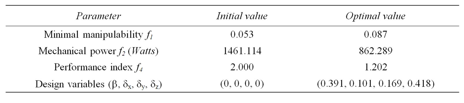
Table 3. Initial and optimal parameter values (for k = 0.5).
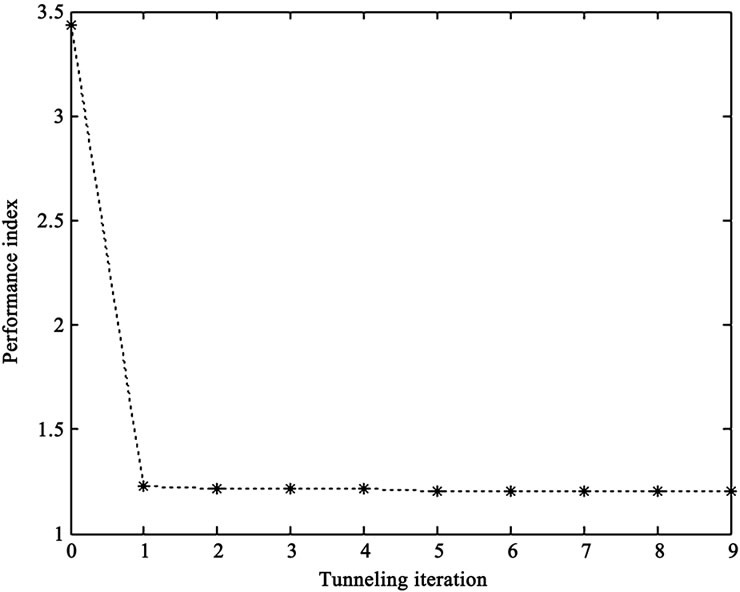
Figure 14. Performance index along the tunneling iterations (for k = 0.5).
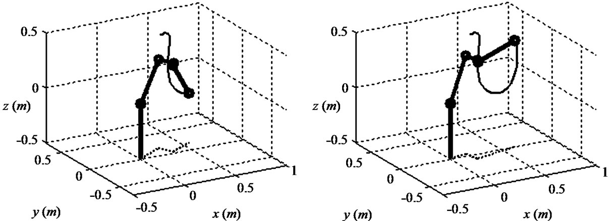
Figure 15. Robot performing the path-following task.
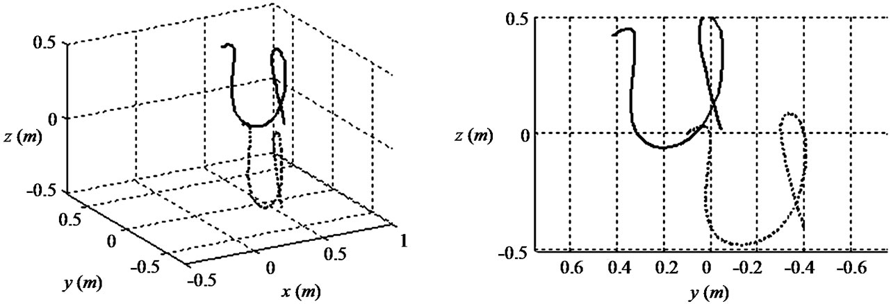
Figure 16. Proposed (---) and optimal (––) paths from two different perspectives.
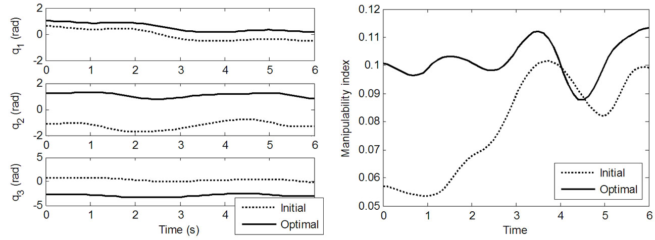
Figure 17. Joint coordinates and the corresponding manipulability index (Puma 560 manipulator).
The joint coordinates at each time step are obtained by inverse kinematics computation. As the task is considered as a set of consecutive Cartesian points with continuous transition, the corresponding joint coordinates presents a smooth behavior. Figure 17 shows the initial and optimal joint coordinates for the first three links and the corresponding manipulability index.
The previous example considered a task initially defined as being parallel to the xz plane, i.e., the path is parallel to a vertical plane. It can be noticed that the optimal design corresponds to rotating the task about 0.391 rad anticlockwise with respect to the reference frame.
8. Conclusions
In this work the path-following problem of robot manipulators was addressed. An approach to increase the manipulability while decreasing dynamics requirements was proposed by using optimization techniques.
The concept of manipulability was revisited. The basic idea behind manipulability analysis consists in describing directions either in the task space or the joint space that optimize the ratio between a measure of effort in the joint space and a measure of performance in the task space. In this work a classical formulation to describe the relation between the two spaces (task and joint spaces) was considered.
Since the end-effector presents various performances due to a number of factors (control specification, joint flexibility, joint friction, etc.), a general methodology to reduce high torques and to increase manipulability was proposed. The corresponding equation considers the overall performance of the entire manipulator, as the determinant of the Jacobian is proportional to the product of its singular values, and the mechanical power index is obtained by a sum involving all the joints. The methodology also includes the manipulator positioning error analysis, through the definition of constraint functions in the optimization model.
The serial manipulator usually performs differently in different zones of the workspace. Considering also the cases for which different joint velocity and torque profiles may result different performance levels, a better position into the workspace (in the sense that the performance indexes are optimized) for performing a specified task was determined.
The optimization problem was based in a global search heuristic, improving the robustness of the process with respect to the initial guess.
Numerical experiments showed that the task repositioning successfully increases the manipulability and reduces the total mechanical power, simultaneously. As changes in the task positioning may result different associated manipulability indexes and different joint velocity and torque profiles, the methodology searches for an optimal way of using the robot possibilities (as described by the performance indexes) by finding an optimal position into the workspace to perform the task.
In some practical cases, the manipulated objects cannot be displaced because of physical constraints such as weight or geometry. Even in such cases the proposed strategy is suitable to be applied by changing the position of the manipulator itself. The corresponding changes in the robot’s base are given by the optimal profile by using the opposite sign of the optimal values, i.e., (-β, -δx, -δy, -δz). It is also possible to adjust the analysis to consider different objectives, as the total torque instead of the mechanical power, for example. The steps to be followed remain the same.
In summary, the main contributions of this paper are the simultaneous analysis of both the required mechanical power and the manipulability (dynamics and kinematics aspects), together with a global deterministic heuristic to achieve the optimal task placement.
As the proposed methodology is suitable for serial manipulators of arbitrary complexity, the authors believe that the present methodology represents a contribution concerning general optimal robot path planning and design.
9. Acknowledgements
The authors are thankful to the agencies FAPEMIG and CNPq (INCT-EIE) for partially funding this work.
10. References
[1] S. F. P. Saramago and V. Steffen Jr., “Optimization of the Trajectory Planning of Robot Manipulators Taking Into-Account the Dynamics of the System,” Mechanism and Machine Theory, Vol. 33, 1998, pp. 883-894.
[2] R. R. D. Santos, V. Steffen Jr. and S. F. P. Saramago, “Robot Path Planning: Avoiding Obstacles,” In: 18th International Congress of Mechanical Engineering, Ouro Preto-MG, Brazil, 2005.
[3] S. S. Chiddarwar and N. R. Babu, “Offline Decoupled Path Planning Approach for Effective Coordination of Multiple Robots,” Robotica, Vol. 28, No. 4, 2010, pp. 477- 491.
[4] R. R. D. Santos, V. Steffen Jr. and S. F. P. Saramago, “Optimal Path Planning and Task Adjustment for Cooperative Flexible Manipulators,” ABCM Symposium Series in Mechatronics, Associação Brasileira de Engenharia e Ciências Mecânicas, ABCM, Vol. 3, 2008, pp. 236-245.
[5] O. Von Stryk and M. Schlemmer, “Optimal Control of the Industrial Robot Manutec r3,” Computational Optimal Control, International Series of Numerical Mathematics, Vol. 115, 1994, pp. 367-382.
[6] R. R. D. Santos, V. Steffen Jr. and S. F. P. Saramago, “Robot Path Planning in a Constrained Workspace by Using Optimal Control Techniques,” In: III European Conference on Computational Mechanics, Lisbon, Portugal, 2006, pp. 159-177.
[7] J. E. Bobrow, S. Dubowsky and J. S. Gibson, “Time-Optimal Control of Robotic Manipulators along Specified Paths,” The Intemational Journal of Robotics Research, Vol. 4, 1995, pp. 3-17.
[8] J. E. Slotine and H. S. Yang, “Improving the Efficiency of Time-Optimal Path-Following,” IEEE Transaction on Robotics and Automation, Vol. 5, No. 1, 1989, pp. 118- 124.
[9] D. Constantinescu and E. A. Croft, “Smooth and TimeOptimal Trajectory Planning for Industrial Manipulators along Specified Paths,” Journal of Robotic Systems, Vol. 17, 2000, pp. 233-249.
[10] H. Seraji, “Reachability Analysis for Base Placement in Mobile Manipulator,” Journal of Robotic Systems, Vol. 12, 1995, pp. 29-43.
[11] S. Zeghloul and J. A. Pamanes, “Multi-Criteria Optimal Placement of Robots in Constrained Environments,” Robotica, Vol. 11, No. 2, 1993, pp. 105-110.
[12] J. T. Feddema, “Kinematically Optimal Robot Placement for Minimum Time Coordinated Motion,” Proceedings of the IEEE International Conference of Robotics and Automation, Minneapolis, 1996, pp. 3395-3400.
[13] F. C. Park, “Distance Metrics on the Rigid-Body Motions with Applications to Mechanicsm Design,” ASME Journal of Mechanical Design, Vol. 117, 1995, pp. 48-54.
[14] G. S. Chirikjian and S. Zhou, “Metrics on Motion and Deformation of Solid Models,” ASME Journal of Mechanical Design, Vol. 120, 1998, pp. 252-261.
[15] J. M. R. Martinez and J. Duffy, “On the Metrics of Rigid Body Displacement for Infinite and Finite Bodies,” ASME Journal of Mechanical Design, Vol. 117, No. 1, 1995, pp. 41-47.
[16] B. Tabarah, B. Benhabib, R. Fenton and R. Cohen, “Cycle-Time Optimization for Single-Arm and Two-Arm Robots Performing Continuous Path Operation,” 21st Biennial Mechanisms Conference, Chicago IL, 1990, pp. 401-406.
[17] Y. Zhang, and K. Li, “Bi-Criteria Velocity Minimization of Robot Manipulators Using LVI-Based Primal-Dual Neural Network and Illustrated Via PUMA560 Robot Arm,” Robotica, Vol. 28, No. 4, 2010, pp. 525-537.
[18] K. Abdel-Malek and W. Yu, “On the Placement of Serial Manipulator,” Proceedings of DETC00 2000 ASME Design Engineering Technical Conferences, Baltimore, MD, 2000, pp. 1-8.
[19] Y. Chen and A. A. Desrochers, “Structure of Minimum-Time Control Law for Robotic Manipulators with Constrained Paths,” IEEE International Conference on Robot and Automat, Scottsdale, Az, USA, 1989, pp. 971- 976.
[20] Z. Shiller and H. H. Lu, “Computation of Path Constrained Time Optimal Motions with Dynamic Singularities,” ASME Journal of Dynamic Systems, Measurement, and Control, Vol. 114, 1992, pp. 34-40.
[21] E. K. Xidias, P. T. Zacharia and N. A. Aspragathos, “Time-Optimal Task Scheduling for Articulated Manipulators in Environments Cluttered with Obstacles,” Robotica, Vol. 28, No. 3, 2010, pp. 427-440.
[22] K. S. Fu, R. C. Gonzales and C. S. G. Lee, “Robo-Tics: Control, Sensing, Vision and Intelligence,” McGraw-Hill, New York, 1987.
[23] T. Yoshikawa, “Manipulability of Robot Mechanisms,” The International Jouranl Robotics Research, Vol. 4, 1985, pp. 3-9.
[24] M. J. Richard and C. M. Gosselin, “A Survey of Simulation Programs for the Analysis of Mechanical Systems,” Mathematics and Computers in Simulation, Vol. 35, No. 2, 1993, pp. 103-121.
[25] V. Mata, F. Benimeli, N. Farhat and A. Valera, “Dynamic Parameter Identification in Industrial Robots Considering Physical Feasibility,” Journal of Advanced Robotics, Vol. 19, No. 1, pp. 101-120.
[26] V. Mata, S. Provenzano, F. Valero and J. I. Cuadrado, “Serial Robot Dynamics Algorithms for Moderately Large Numbers of Joints,” Mechanism and Machine Theory, Vol. 37, No. 8, pp. 739-755.
[27] J. J. Craig, “Introduction to Robotics: Mechanics & Control,” 2nd Edition, Reading, MA: Addison-Wesley, 1989.
[28] R. R. D. Santos, V. Steffen Jr. and S. F. P. Saramago, “Solving the Inverse Kinematics Problem through Performance Index Optimization,” In: XXVI Iberian Latin-American Congress on Computational Methods in Engineering, Guarapari-ES, 1985.
[29] H. Eschenauer, J. Koski and A. Osyczka, “Multicriteria Design Optimization,” Springer-Verlag, Berlin, 1990
[30] G. N. Vanderplaats, “Numerical Optimization Techniques for Engineering Design,” 3rd Edition, VR & D Inc., 2001.
[31] A. V. Levy and S. Gomez, “The Tunneling Method Applied to Global Optimization. Numerical Optimization,” (Ed. P. T. Boggs) R. H. Byrd and R. B. Schnabel, Eds., Society for Industrial and Applied Mathematics, 1985, pp. 213-244.
[32] A. V. Levy and A. Montalvo, “The Tunneling Algorithm for the Global Minimization of Functions,” The SIAM Journal on Scientific and Statistical Computing, Vol. 6, No. 1, 1985, pp. 15-29.
[33] D. G. Luenberger, “Linear and Nonlinear Programming,” 2nd Edition, Addison-Wesley, USA, 1984.
[34] G. N. Vanderplaats, “An Efficient Feasible Direction Algorithm for Design Synthesis,” American Institute of Aeronautics and Astronautics Journal, Vol. 22, No. 11, 1984, pp. 1633-1640.
[35] G. N. Vanderplaats, “DOT-Design Optimization Tools Program,” Vanderplaats Research & Development, Inc., Colorado Springs, 1995.