Positioning
Vol.4 No.4(2013), Article ID:39553,11 pages DOI:10.4236/pos.2013.44027
A Robust Hybrid Multisource Data Fusion Approach for Vehicle Localization
![]()
The French Institute of Science and Technology for Transport, Development and Networks (IFSTTAR), COSYS Department, LIVIC Laboratory, 77 rue des Chantiers, Versailles, France.
Email: adda-redouane.ahmed-bacha@ifsttar.fr, dominique.gruyer@ifsttar.fr, alain.lambert@ifsttar.fr
Copyright © 2013 Adda Redouane Ahmed Bacha et al. This is an open access article distributed under the Creative Commons Attribution License, which permits unrestricted use, distribution, and reproduction in any medium, provided the original work is properly cited.
Received August 16th, 2013; revised September 16th, 2013; accepted September 23rd, 2013
Keywords: Localization; Mobile Robotic; Kalman Filter; EKF; Particle Swarm Optimization; PSO; Particle Filter; Data Fusion; Vehicle Positioning; Navigation; GPS
ABSTRACT
In this paper, an innovative collaborative data fusion approach to ego-vehicle localization is presented. This approach called Optimized Kalman Swarm (OKS) is a data fusion and filtering method, fusing data from a low cost GPS, an INS, an Odometer and a Steering wheel angle encoder. The OKS is developed addressing the challenge of managing reactivity and robustness during a real time ego-localization process. For ego-vehicle localization, especially for highly dynamic on-road maneuvers, a filter needs to be robust and reactive at the same time. In these situations, the balance between reactivity and robustness concepts is crucial. The OKS filter represents an intelligent cooperative-reactive localization algorithm inspired by dynamic Particle Swarm Optimization (PSO). It combines advantages coming from two filters: Particle Filter (PF) and Extended Kalman filter (EKF). The OKS is tested using real embedded sensors data collected in the Satory’s test tracks. The OKS is also compared with both the well-known EKF and the Particle Filters (PF). The results show the efficiency of the OKS for a high dynamic driving scenario with damaged and low quality GPS data.
1. Introduction
Localization of vehicles is a research topic in perpetual evolution. Nowadays, the location information becomes very important and inevitable in large cities in order to move from point A to a desired point B. Developing the localization to produce new services increasing the drivers’ safety and autonomy becomes the logical continuity. Researchers aim to develop more accurate positioning than only the positioning obtained with natural global positioning system with the use of satellites constellation. This new type of positioning opens fields for new Intelligent Transport Systems applied to Road applications (ITS-R) and advanced systems for driving assistance (ADAS) such as parking valet, and copilot for autonomous driving. However, the development of new services using an accurate localization should have a slight impact from an economic point of view. For this reason, research was directed toward hybrid fusion methods which consisted in using of onboard sensors or new low cost sensors. These sensors bring new information allowing better estimation of the vehicle position with a high confidence. There is a wide range of research works using the GPS data for ego-vehicle localization applications. Other sensors such as inertial navigation system (INS), Odometer, and wheel steering angle sensor are used for dead reckoning localization process development [1-3]. Estimating a vehicle location in Mobile Robotics consists of determining both vehicle position and orientation relatively to its environment. The vehicle localization problem is considered in the mathematic-probabilistic field [4,5] as a state estimation problem. Accurate vehicles models are generally nonlinear. It is very difficult to use the Kalman Filter (KF) in practice, because it is an optimal filter only for linear systems [6]. Data fusion based filtering approaches are mostly non-linear Kalman variants [3,7-9]. To bypass the model nonlinearity problem, the Extended Kalman Filter (EKF) based localization has been proposed for autonomous vehicles positioning such as in [10-12]. Particle Swarm Optimization (PSO) is a metaheuristic optimization method attributed to Eberhart, Shi and Kennedy [13]. Improved for optimization issues [14-17], the PSO introduces social behaviors and cognitive concepts to the localization process. With these notions, particles are directed toward the high probability positioning region of the state space (sensor information). Samples move in the direction of their best neighbor (social communication) to finally converge to local optima or global optimum. The development of localization applications inspired by PSO has risen within the last years, inspiring hybrid approaches such as the Swarm particle filter (SPF) and PSO aided Kalman filter [1,18,19]. The SPF consists in an integration of the PSO to the Particle Filter. This integration allows applying the optimization technique to tracking and localizing applications. The SPF then represents an interesting approach to localization, but it still has premature convergence and parameterization problems. The PSO also is used in [19] to tune Kalman process noise in order to avoid Kalman filter limitation for abrupt dynamic changes. The PSO aided Kalman filter becomes then too time-consuming and needs PSO parameters tuning.
This paper presents a new localization approach. Inspired by the following localization and tracking research works [1,18,19], this vehicle localization method is called the Optimized Kalman Swarm (OKS). The OKS performs the positioning process considering a dynamic optimization problem. Explicitly, at each step, the OKS method tries to find the best possible vehicle position according to the GPS measure, the predicted vehicle state and the relayed information between particles.
A comparison is made using the same real word experimental data and noises for all approaches (EKF, PF and OKS). Filters performances are evaluated to rank them in terms of accuracy and robustness. A centimetric RTK GPS is used as a reference trajectory. Also, investigations on the filters uncertainty ellipses areas are done to evaluate filters’ uncertainty. The tests will also compare the filters behavior depending on GPS quality information cases (good, noisy, multi-path or missing signal).
The reminder of the article will be organized as follows: Section 2 is dedicated to a background part; this item presents the theoretical and algorithmic foundations of the approaches inspiring the OKS. It begins by a presentation of the particles based approaches. Section 2.1 introduces the PSO algorithm and the Particle Filter giving details of their different algorithmic steps, while the EKF is detailed in Section 2.2. The OKS is then presented and detailed in Section 3, in order to carry out a theoretical and experimental filters comparison and analysis in Section 4. Conclusion about this work is given in Section 5. In the last section, some future works and improvement ways are proposed.
2. Backgrounds
This section provides an overview of the methods used as the foundation of the OKS on-road vehicle localization approach.
We will start with an overview of the Particle Swarm Optimization. Then, we will present the Particle Filter (PF) approach. The Particles approaches represent a famous alternative to the Bayesian ones with the advantage to be more resistant to noises. The third and last part will introduce a classic Bayesian method which is the Extended Kalman Filter (EKF). This filter and its variants represent the mostly used Bayesian techniques in the localization field.
2.1. PSO and PF Overview
2.1.1. Particle Swarm Optimization Basics (PSO)
First intended for simulating social behaviour and originally attributed to Eberhart, Shi and Kennedy [13]. The Particle Swarm Optimization is based on a set of samples called particles initially arranged randomly and homogeneously in the search space. Each particle moves in the search space and represents a potential solution of the processed problem. Each particle is equipped with a memory that allows it to know its best found solutions. Moreover, each particle has the capability to communicate with its environment (neighborhood), that gives the position of the best solution ever found by its informants. Using this information, each particle is going to move by updating its evolution state vector. The evolution (motion) of a particle is affected by three behaviors: First, a tendency to keep its own way called selfish. The second tendency makes the particle reverting to its best found solution and is known as the Conservative behavior. Third and last one is the Herding (Social, Collective) behavior, which exhorts the particle to move towards the best informant (neighbor) which represents the best current solution found by its neighborhood. These tendencies (behaviors) are illustrated in Figure 1. The selfish tendency is weighted by the inertia weight W, while the two remaining tendencies can be weighted with learning factors, random weights or the both, depending on the PSO variant.
Particles have some attributes. At time t the particle (sample) i is caracterised by the following:  is the position in the search space noted by a state vector. The state vector values depend on the processed system and the application. Here we use the same state vector for all approaches which is the position-orientation vector
 .
.  is the particle speed, it represents the displacement of a particle
 .
.  is the state vector of the best solution covered by the par-
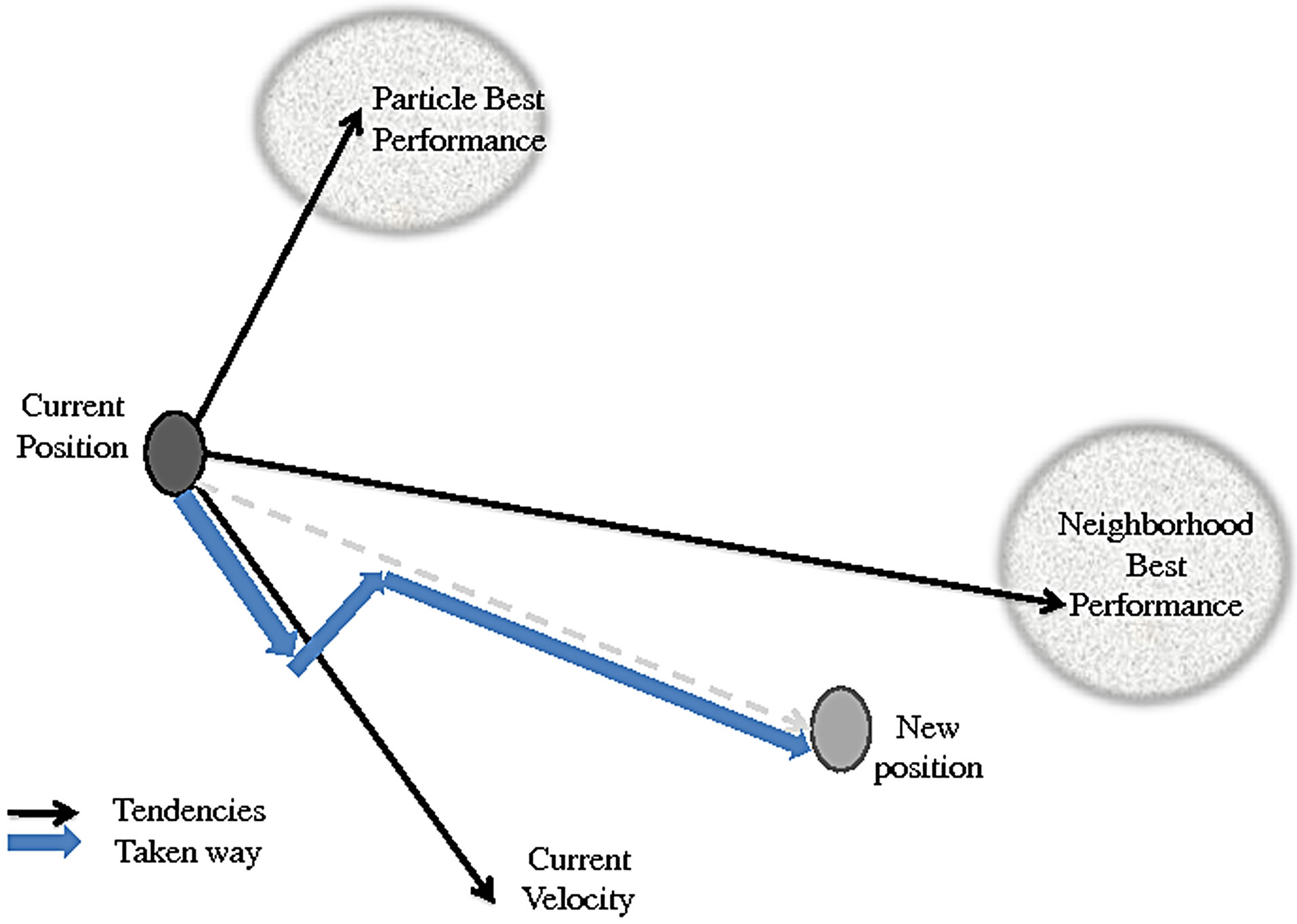
Figure 1. PSO Particle motion.
ticle, it is given by the best saved score that this particle has reached. And  represents the best neighborhood solution, it is a state vector given by scores comparison among all the communicative neighbors (informants). The communicative neighbors can represent all the swarm or selected particles from the swarm depending on the neighborhood topology and size. The more the neighborhood is informative the more information is shared and convergence is enhanced. An example of a geographical neighborhood is shown in Figure 2. It is based on the nearby particles and must be calculated at each iteration, while Figure 3 presents some social neighborhood configurations. This kind of neighborhood is set at the beginning and does not require distance calculation to find the neighbors. In case of convergence, the social neighborhood tends to become geographical.
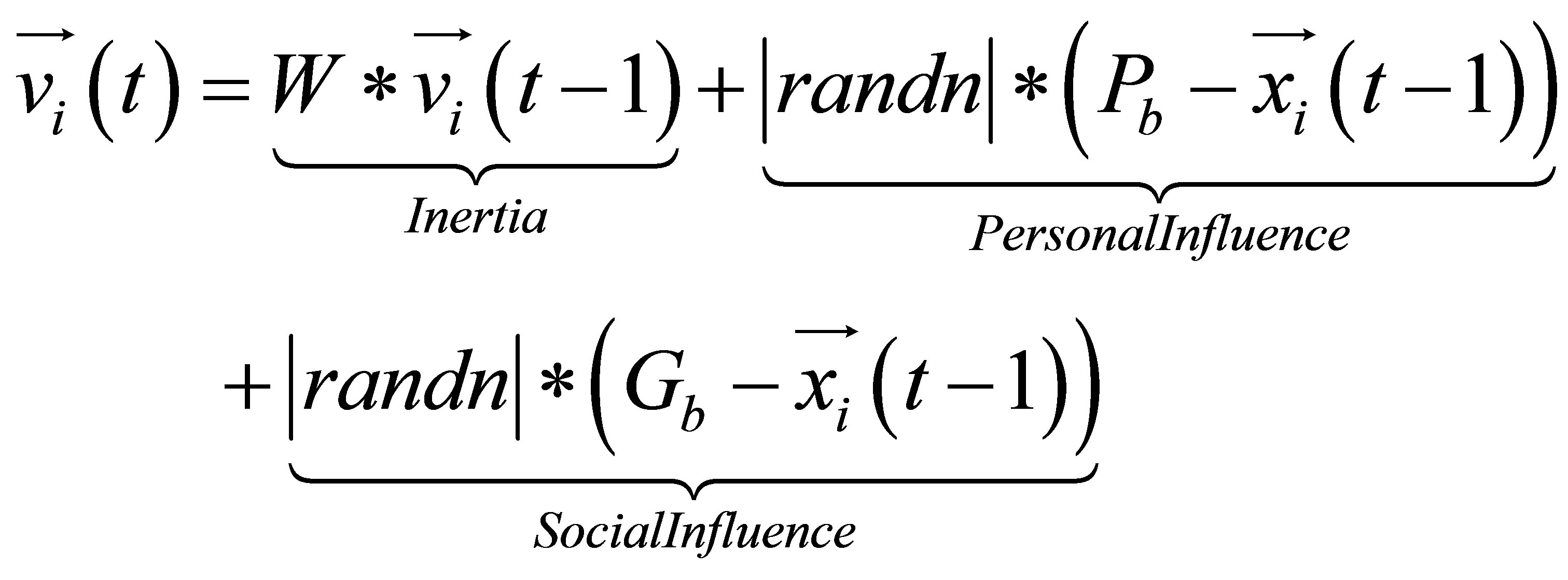
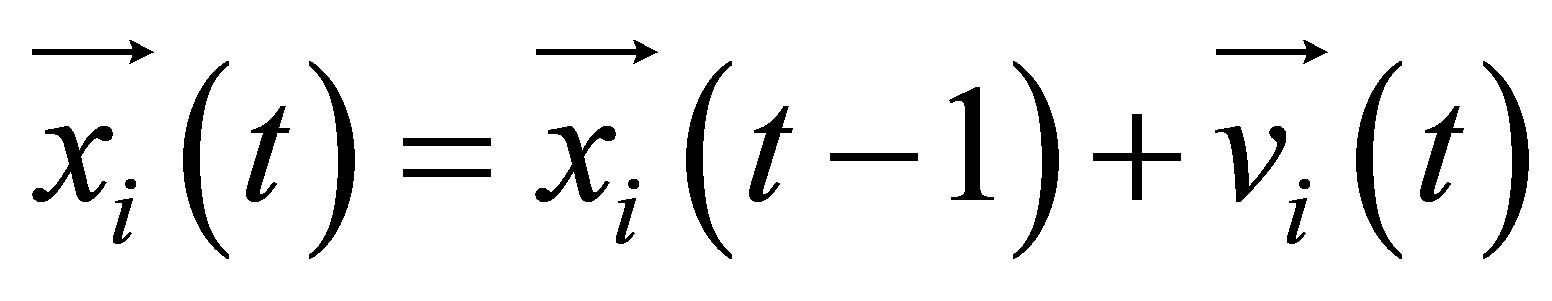
The optimization depends essentially on the evolution of particles. The evolution consists in changing position by the application of a calculated speed using the weighted three influencing tendencies:
 (1)
(1)
 (2)
(2)
Some variants of these evolution equations are available in [13,18,20,21]. Each variant of the evolution equations is designed to assist with the balance between exploration and convergence during the optimization process, see [22,23] for evolution variants comparison. The Equations (1) and (2) are inspired by the Gaussian swarm variant which is based on the Gaussian distribution to improves the convergence ability of the PSO without the necessity of tuning factors [21].
From local optima, the swarm of particles will con-
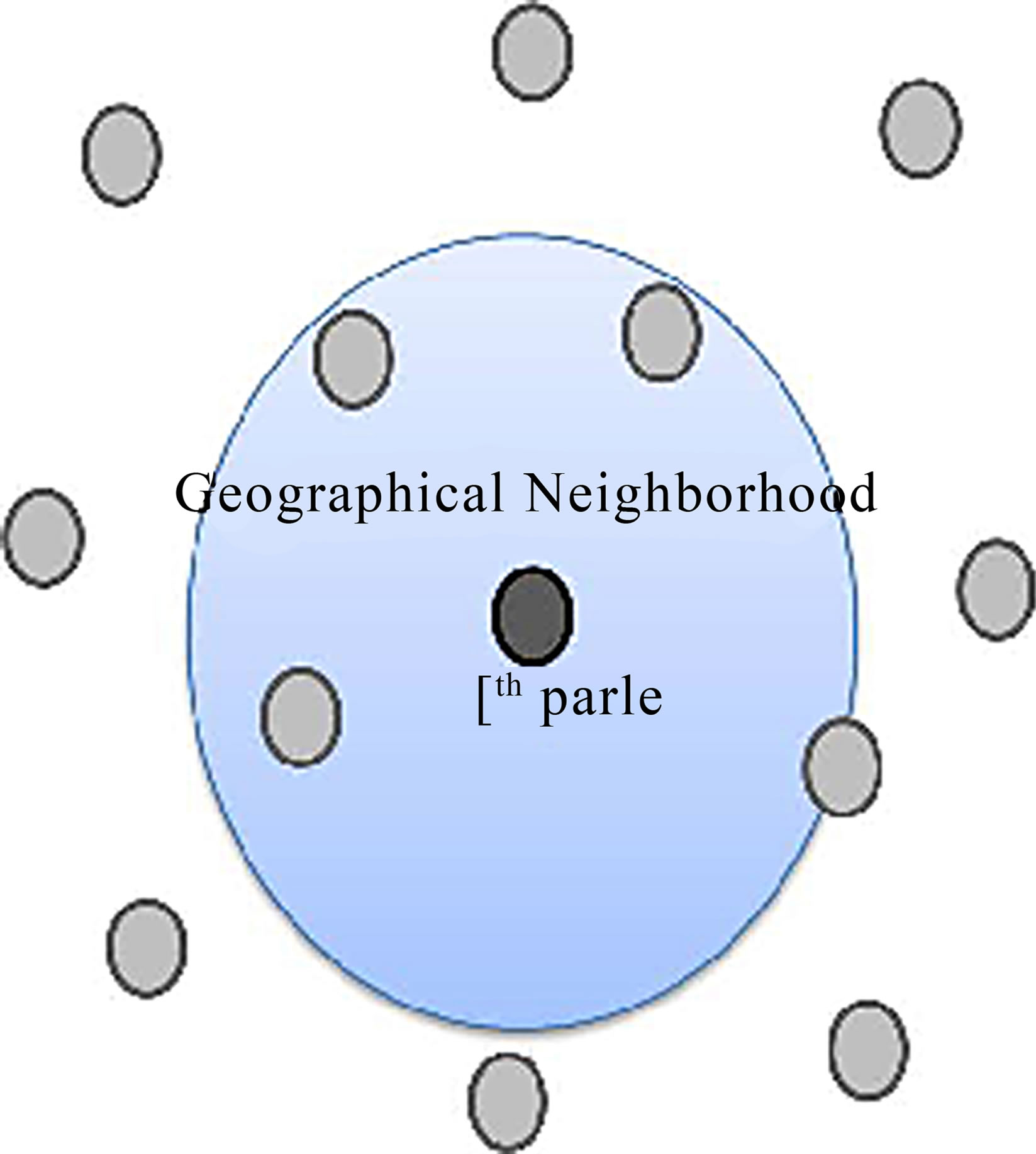
Figure 2. Diagram of a geographical neighborhood.
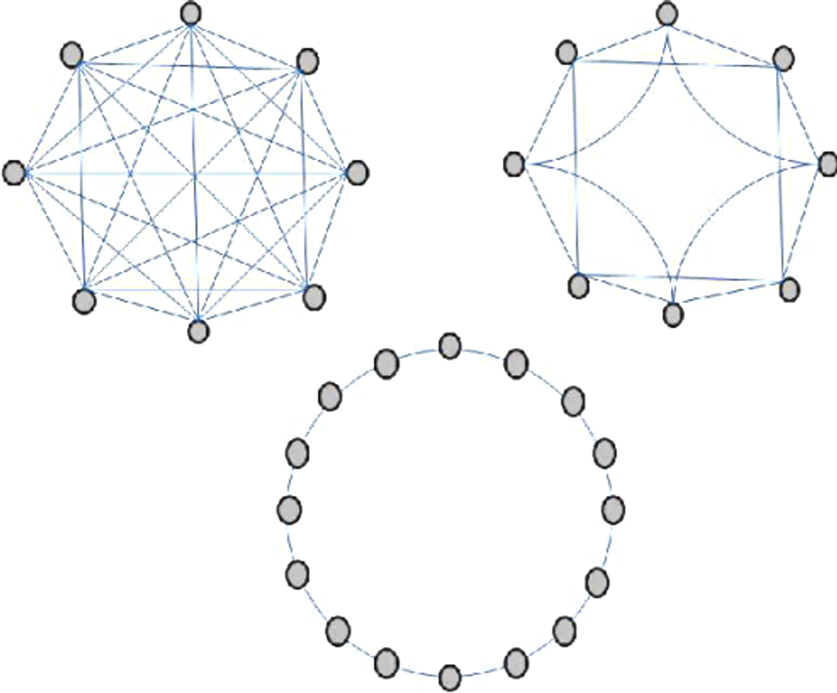
Figure 3. Different configurations of social neighborhood (from top to bottom and from left to right): Star, ring, and circle.
verge to a global optimal solution of the problem. The algorithm of a basic Particle Swarm Optimization process is stated in Figure 4.
2.1.2. The Particle Filter (PF)
The particle filter (sequential Monte-Carlo method (SMC)) is a numerical method to approximate the probability distribution of the state by means of the empirical distribution of particles. Each particle represents a possible configuration of the estimated state. A weight is affected to each particle in order to judge the consistency of the sample according to the conditional probability of the state while experiencing the observations. The particle filter can be faster than the Monte-Carlo Markov chains. It is often an alternative to the extended Kalman filter with the advantage that with sufficient samples, it ap-
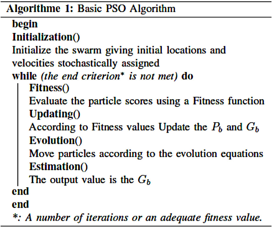
Figure 4. Basic PSO Algorithm.
proaches the optimal Bayesian estimate. The PF can be made more accurate than Kalman filters, it remains to do a compromise between computational time and accuracy.
The EKF and PF approaches can be combined using the Extended Kalman filter to give a prior estimation (prediction) for the particle filter using an evolution model as an alternative of random evolutions by adding noises. To combine techniques assets, hybrid localization approaches are processed these last few years.
The particle filter algorithm is detailed in the following:
1) Initialization:
In order to localize a vehicle during a driving test, we consider an initial position of the vehicle represented by the state vector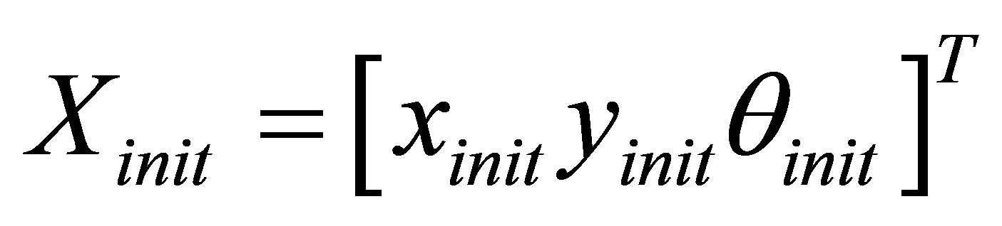 . Then, the initial cloud of samples is drawn around this initial position by assigning each particle a state vector X and an initial weight w. The number N is the number of particles (samples) and is to be determined by the user. The state vectors of the particles represent a Gaussian distribution centered on the initial position according to this model:
At the initialization step each particle i has a state vector 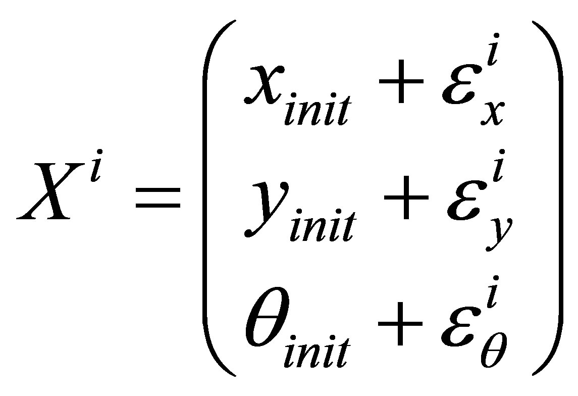 and a weight
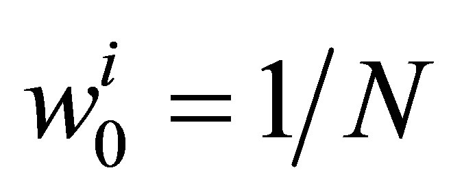 .
.
The 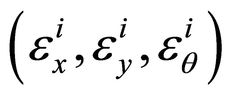 are random variables, these errors are added to represent the initial state in the form of a gaussian cloud of particles scattered across the search space around the initial position according to its uncertainty. The centered normal laws of probability used in this case are
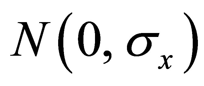 ,
,  ,
,  where
where  are taken from the initial variance-covariance matrix of noise.
2) Prediction:
Here, from the last known position of the vehicle  and available data from proprioceptive sensors such as INS, wheel steering angle encoder and odometer, we calculate a predicted position of the vehicle
 . This position represents the vehicle condition assumed at this moment. It is calculated using a vehicle model incorporating proprioceptive sensors data and their respective uncertainties (the used model in all tests will be a bicycle vehicle model). The dynamic model of the vehicle (evolution matrix) is applied to each particle in order to obtain a new state vector
  (a predicted state vector). It is important to integrate to this prediction step the measurement errors and evolution errors. These noises allow each particle to move in a different way, this encourages the exploration of the search space. If the noise is too low, the filter will not work well and particles will not represent enough noise condition or uncertainty around the predicted state for this case. If the noise is too high, the filter may diverge due to excessive scattering of particles on several consecutive steps.
3) Update:
This step is performed to reassess (Update) the weights of particles using exteroceptive sensors data such as GPS, visual information, and/or mapping. For updating, we adjust our prediction by revaluating the particles weights according to a new GPS data while taking into account the different uncertainties. This can be considered as conciliation between a predictive datum and a corrective one. The weights calculation is done following the Equation (3).
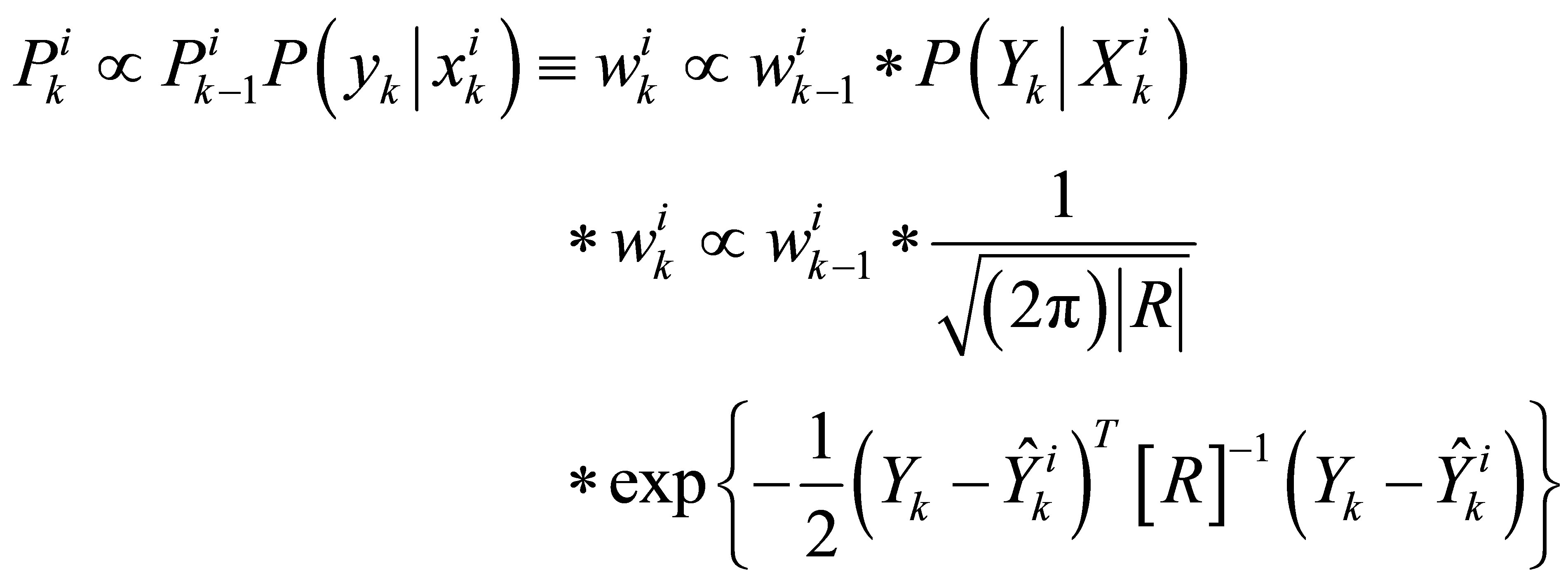 (3)
(3)
4) Normalization and Estimation:
After updating weights, in order to keep the sum of the probabilities equal to 1, a normalization of the particles weights is performed according to the Equation (4).
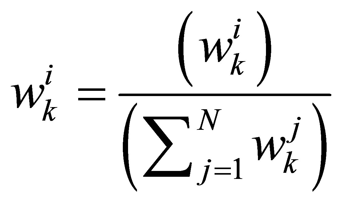 (4)
(4)
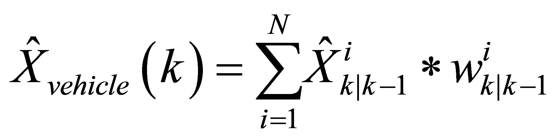
After the normalization of weights, the vehicle position is calculated with the fusion Equation (5):
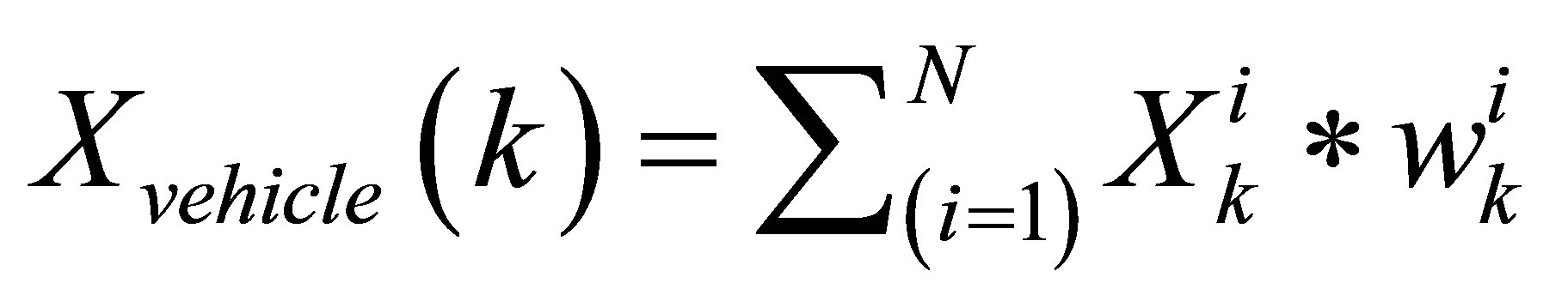 (5)
(5)
5) Resampling:
Resampling is a critical step for the proper functioning of the swarm particle filter approach. It prevents the divergence and degeneracy of the filter by eliminating low weight particles and duplicating those with interesting weights.
There are a multitude of approaches for resampling as well as resampling criterions, see [24] for more details. The used algorithm is the systematic resampling one with the Kong criterion (6) for its enabling/disabling:
 (6)
(6)
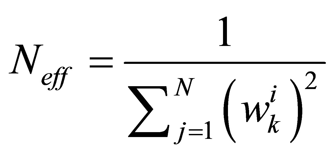
Where  is the standardized weight of the particle i at time k.
 tends to M when the distribution of the particles weights is efficient.
 tends to 1 when the distribution of the particles weights is inefficient.
The resampling is performed if  is under the defined threshold
 . This threshold represents the minimum of required effectiveness, it is generally a fixed value within this range
  i.e.
i.e.  with N the number of particles and α a term representing the minimum desired percentage of consistent particles, for eg. α = 0.5 for 50% of minimum effective particles. After the resampling step, all particles weights are set to
 .
.
The Swarm Particle Filter (SPF) is a hybridization of the PF with an integration of the social influence of the PSO. An approach inspired by Particle filter hybridization with Particle Swarm Optimization (PSO) is expected to make use of the interactivity aspect in addition to the reactive aspect of the particle filter. Particles, as for a normal Particle Filter, go through all the particle filter steps. One stage is added. After the update stage, particles exchange information (communicate) and evolve in order to optimize the swarm distribution (move toward the region where the best solutions are found) complying with PSO evolution concept. The SPF suffers generally from premature convergence or swarm explosion problems. These problems are due to the parameters tuning by the user.
2.2. Extended Kalman Filter (EKF)
The Extended Kalman Filter (EKF) is the nonlinear version of the Kalman Filter (KF). In the case of well-defined models of evolution, EKF is the most widely used for state estimation for nonlinear navigation systems based on GPS. The Extended Kalman Filter is a recursive estimator. To estimate the current state, only the previous estimate and the current measurements are necessary. The filtered estimate is represented by two terms:  is the state at time k and
  is the covariance matrix representing the estimation uncertainty (a measure of the accuracy of the estimated state). The Kalman filter has two distinct phases: Prediction and Update. The prediction uses the estimated state of the previous time to produce an estimate of the current state. In the update step, the observations of the current time are used to correct the predicted state in order to obtain a more accurate estimate. The EKF implementation begins with an initialization step giving initial values to the following: X: State vector
 . U: Command vector. P: Variance/Covariance confidence matrix. μ: Process noise. Q: Variance/covariance matrix representing the process noise. v: Measurement noise. R: Variance/covariance matrix representing the Measurement noise. Y: Measures Vector.
1) Initialization:
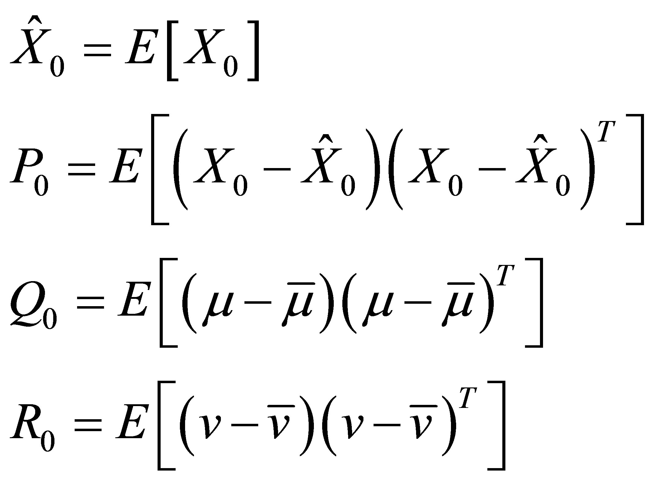 (7)
(7)
2) Jacobians:
The Jacobian matrices are matrix of partial derivatives. A and H are derived respectively from f: the transition or evolution function and h: the observation function. The prediction is made using the evolution matrix A. Then, the update is made with the Kalman gain which is calculated using the measurement matrix H to adjust the state X and reassess the uncertainty P.
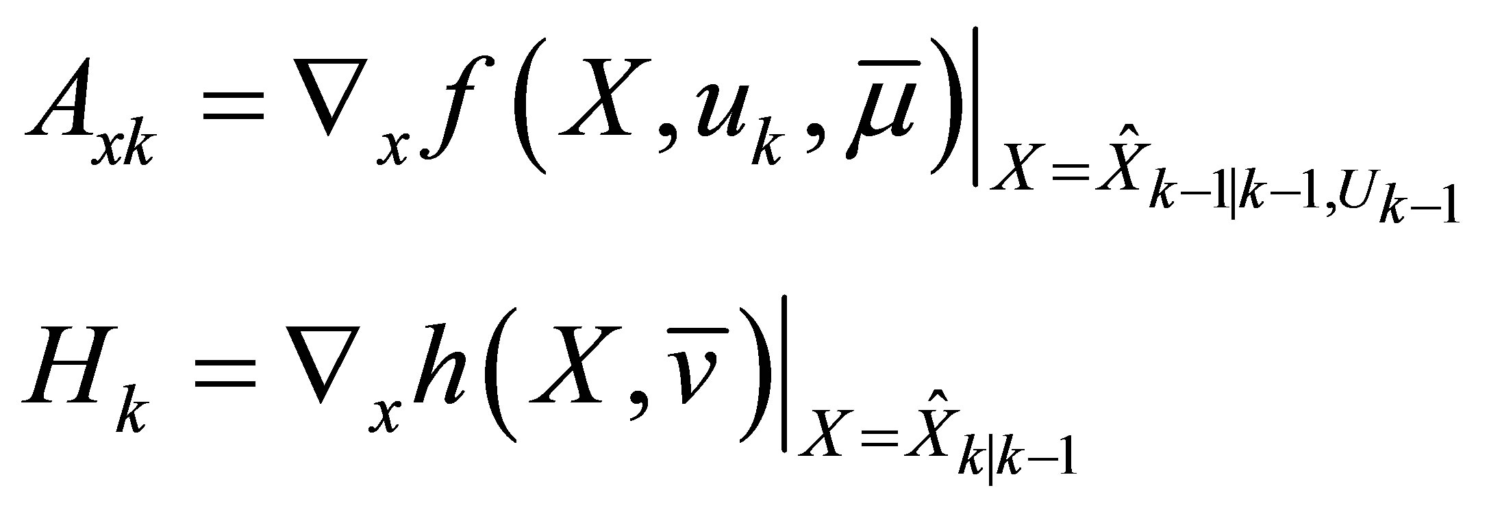 (8)
(8)
3) Prédiction:
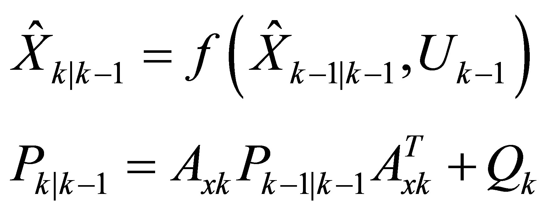 (9)
(9)
4) Update:
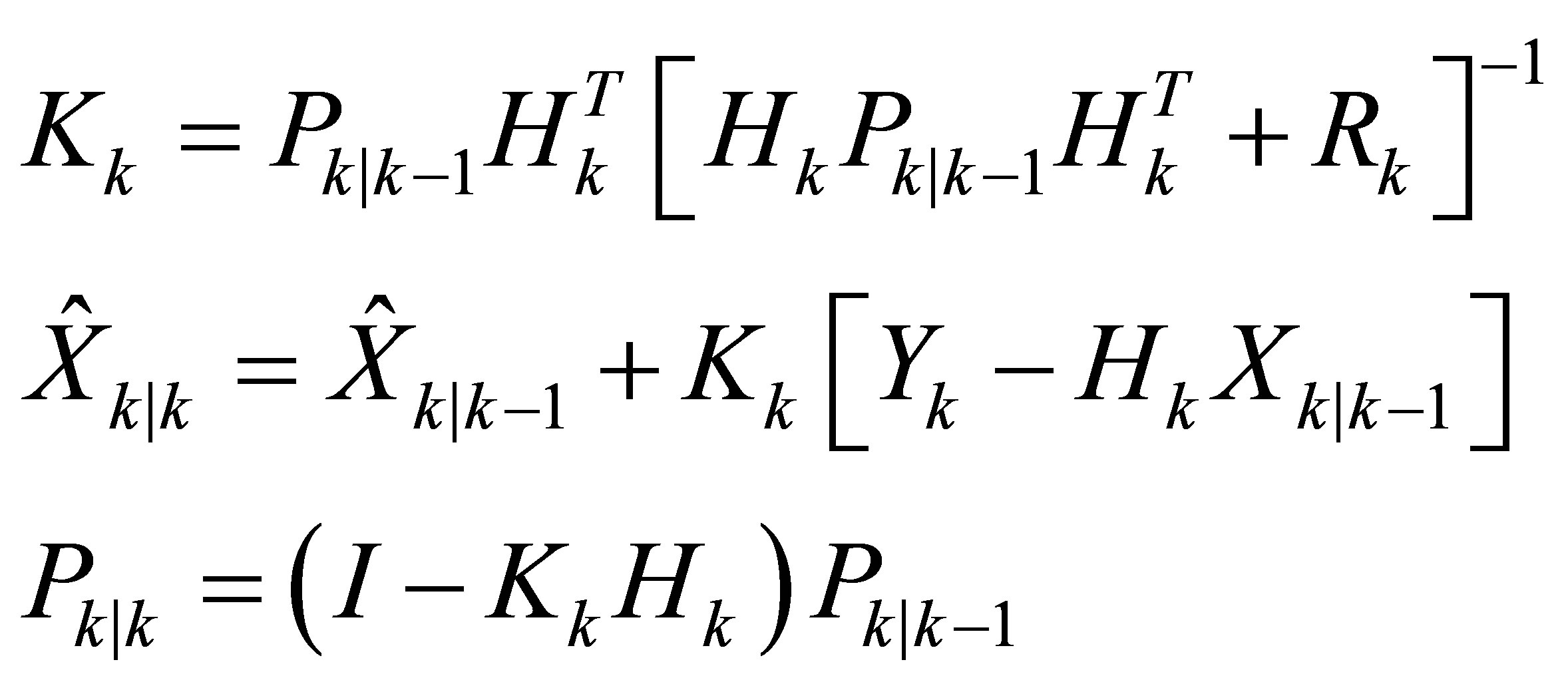 (10)
(10)
3. The Optimized Kalman Swarm (OKS)
The OKS is an evolved version of the SPF. This new filter integrates in addition to the social concept a cognitive one. This last concept is introduced by an adaptive weighting function, called fitness function. The fitness function is managed by the EKF gain in order to be as representative as possible of the particle current probability. The OKS solves the SPF premature convergence problem using less user depending parameters.
3.1. OKS Implementation
The aim of this new approach is to combine the conveniences of the presented techniques in background section, in order to perform an optimization-filtering approach capable of being reactive and cooperative. The cooperative aspect comes out in the OKS with the information exchanging and interaction between particles. The reactive aspect can be found in the capacity of detecting changes in the vehicle’s dynamic. The OKS is then able to be reactive-cooperative. The idea is performed by enhancing particles with a probability matrix (inspired by  of the EKF method) allowing to evaluate the likelihood of each sample. However, this matrix has to be significant and has to represent as well as possible the particle positioning uncertainty. It is the reason why this matrix is managed (updated at each step) with the Extended Kalman filter gain K. During the tracking, particles interact and move following particle swarm optimization concept in order to obtain optimized results and uncertainties. The OKS algorithm can be considered as an evolved SPF hybrid approach aided by a Kalman gain to reassess the likelihood used in an adaptive fitness function.
The algorithm follows the steps described in the flowchart presented in Figure 5.
1) Initialization:
This stage is performed in the same way as the PF initialization. Note, that in addition to all PF particles attributes, a probability matrix is added to each particle and is initialized as an EKF variance confidence matrix. The resulting initialized swarm is done as the following:
After parameters (number of particles M, inertia weight W and resampling factor α) fixing the initial position is calculated with the available data giving , P0, Q0 and R0 values (calculation described in 7). The swarm is then initialized following the PF intialization 2.1.2.a.
An initial OKS particle has these attributes:  which is a state vector
  integrating initial sensors and model noises.
  is an initial speed value set to 0.
  represents the particle initial uncertainty matrix. And an initial score value
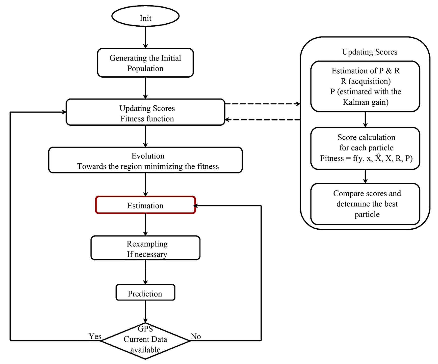
Figure 5. OKS algorithme.
 which will be updated after using the fitness function (12).
  and
and  are swarm attributes representing the initial best personal and global solutions.
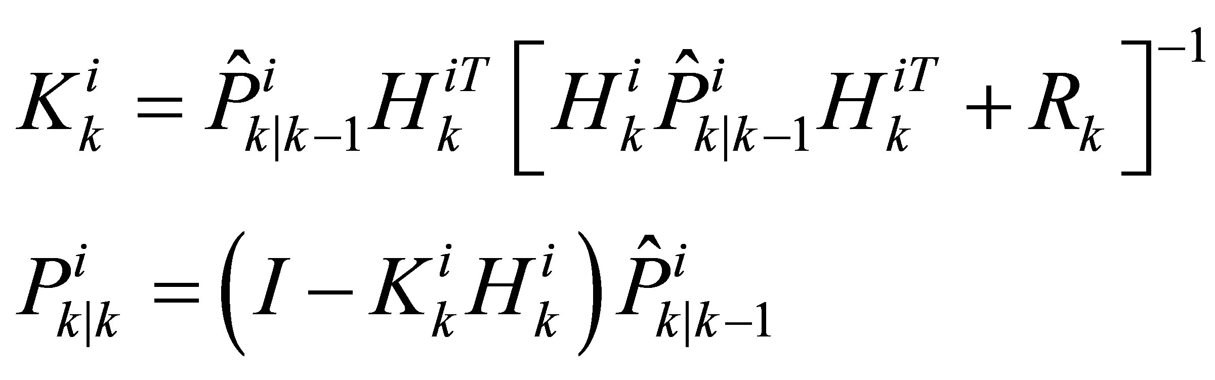
2) Prediction:
Each position sample (particle’s state vector) is passed through the vehicle bicycle evolution model by integrating the system noise to the matrix  (the confidence variance-covariance matrix of a particle) according to the EKF prediction Equations (9),
  and
and  .
.
A predicted vehicle state vector is then provided by the weighted mean of the predicted particles states vectors
 .
.
3) Updating Scores:
For the scores evaluation, the matrix  is updated using a Kalman gain to be as representative as possible of the particle i uncertainty. Also the matrix R using the data of the GPS signal quality is updated with the new available data acquisition. The update of
  is made according to the Equation (11):
 (11)
(11)
The score for each particle is calculated with the Fitness function detailed in the following.
The Fitness function is a minimization or maximization criterion reflecting one or multiple goals of our optimization, the selection of this function depends on the application and the desired result [14,17, 23].
The developed fitness function 12 describes a score calculation representing a criterion to be maximized. The calculated score represents information squared errors respectively weighted with their uncertainties. This function considers two information sources: the prediction information incorporating all proprioceptive sources (Steering wheel angle sensor, Gyrometer and Odometer) and the GPS exteroceptive source.
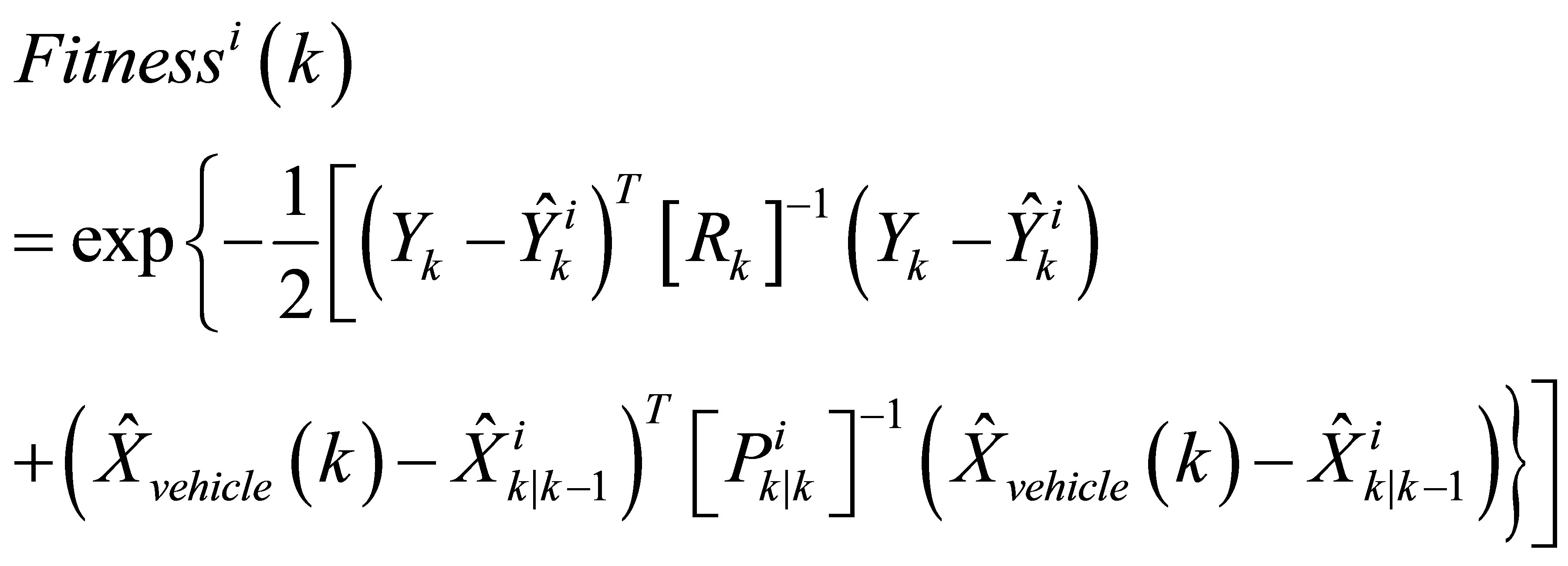 (12)
(12)
 is the predicted measure.
  is the GPS measure,
  represents the GPS uncertainty and
  the estimation uncertainty.
  is the predicted vehicle state. The
  is determined by comparing the particles’ scores.
4) Evolution:
By using the evolution equations presented below, a new position  (state vector) of each particle i is estimated following 13.
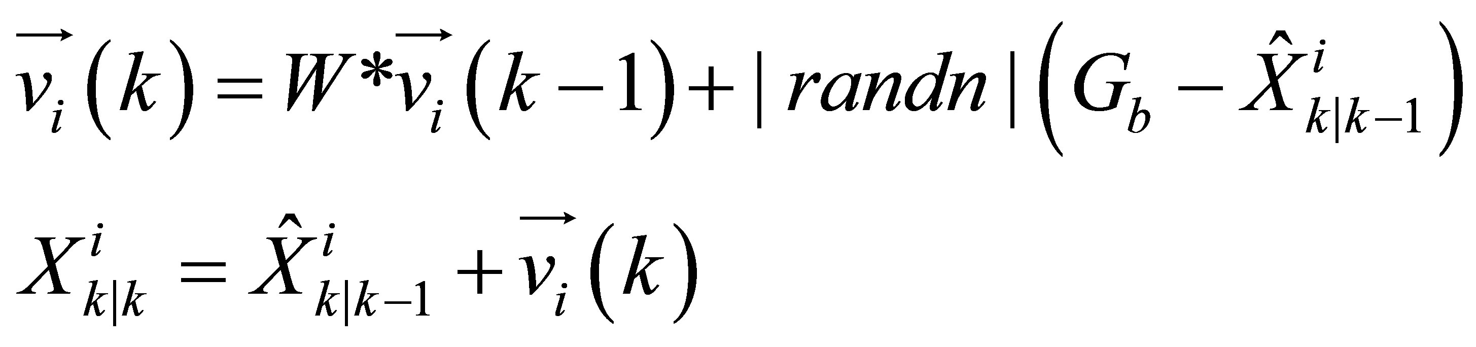 (13)
(13)
The choice of erasing memories of the particles is taken by considering the optimization in a dynamic environment ( is set equal to the particle current position). Such as in the literature approaches addressing dynamic optimization problems [23]. The PSO equation of evolution (2) gives then the OKS evolution Equation (13).
In order to bypass the premature convergence problem, some particles are deprived of the neighborhood information in order to provide behavior diversity. For this, we can fix from the beginning the communicative particles and the free ones or chose randomly at each step.
5) Estimation:
The estimation step is performed by fusing the particles states calculating an estimated vehicle state noted as the weighted mean of particles.
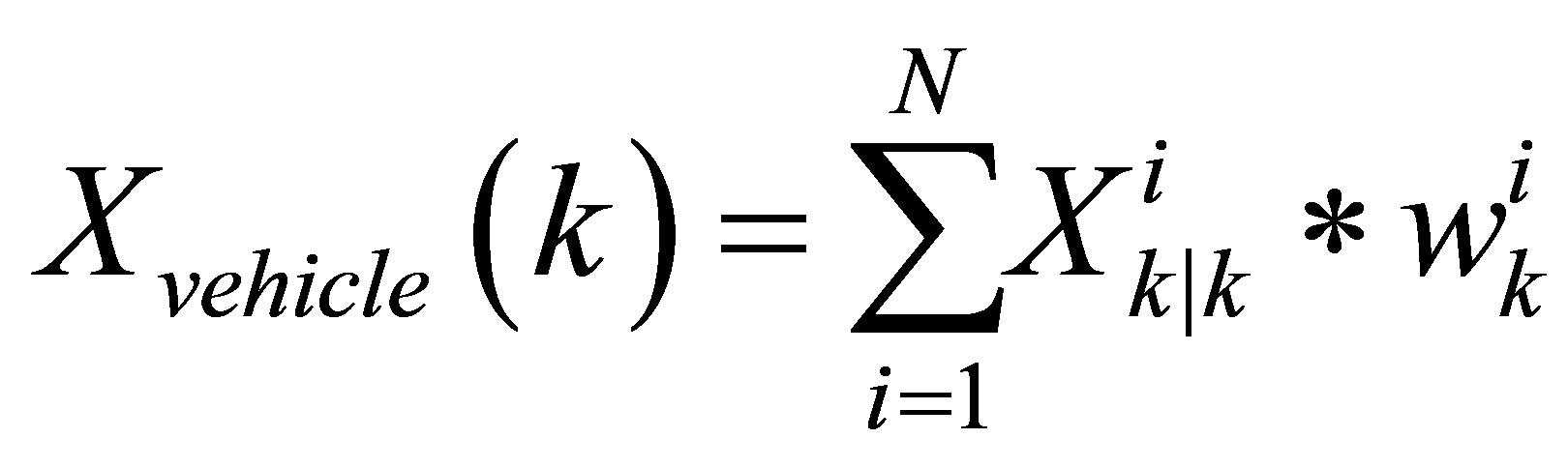
Particles current weights are calculated using the Equation (3) and normalized before the vehicle state estimation.
6) Resampling:
In this process, as for the PF, the resampling is performed using the criterion of Kong, conditioned by the minimum effectiveness threshold Nth. This condition measures the ability of all particles to represent the true position with its posterior probability.
The less the particles population is resampled the more the estimation characteristics of the system’s dynamic are preserved. As the environment is dynamic, the swarm tends to be inefficient from a step to the next one. But it conserves the dynamic of the vehicle (motion and uncertainties) and can become efficient and more informative in next steps. This is especially the case in areas with dynamic changes (ie. start and end of turns). For example, at the beginning of a turn, most of particles conserves straight driving dynamic and are not sufficiently efficient for a turn dynamic motion. After some moves (steps) in turn dynamic, the majority of particles will be tuned for turn estimation and become efficient for this dynamic. The swarm inefficiency will comes out at the straight driving recovery. Then, it is more interesting to have a resampling triggering in these cases (dynamic change) than in the same dynamic running cases. The advantage to preserve free non evolutive particles is then a good solution to guarantee the swarm integrity and heterogeneity.
4. Results Analysis
The purpose of this section is to show strengths and weaknesses of the OKS new approach presented previously. The targeted performances are the robustness and the accuracy. They will be studied in comparison with the EKF and PF.
To achieve a fair-minded comparison, the tests are carried out with the same noises configuration and using the same real sensors data with the same initial configuration. Real data are collected using an equipped vehicle (embedded sensors and dedicated software) of the LIVIC/ IFSTTAR laboratory; the data are collected during real driving tests on the urban area of the Satory test track, see Figure 6. For particles based approaches, the same number of particles (500) is used. The errors calculation will be done by comparing the approaches estimations in comparison with a reference data from a centimetric RTK differential GPS. The inertia weight W is set to 0.2 and the resampling threshold Neff is set to a minimum of 50% effective particles while the average percentage of communicative particles is 10% of the swarm. To test the robustness, we use a database provided by an AG132 GPS running in degraded mode. This database is characterized by a strong noise occasioned by multipaths and/or signal outage. For all tests, the filters variance is high at first (due to pessimist initialization stage) and decreases during the test progression (data accumulation with vehicle traveling) increasing the confidence until it is disturbed by GPS unavailability or an outlier, once the disturbance passes the variance starts to decline again. The studied filters will be compared in terms of accuracy and robustness. The filters performances will be stated by using the RMSE (Root Mean Squared Error) shown in graphics and the mean of axial standard deviations given in tables. The graphics will describe the filters behavior at each step of the test, while the tables will resume the general performance by mean values of axial errors and standard deviations.
The first test is done with a synchronous acquisition of sensors data. The results of the AG132 synchronous test are shown in Figure 7 and Table 1. This figure describes
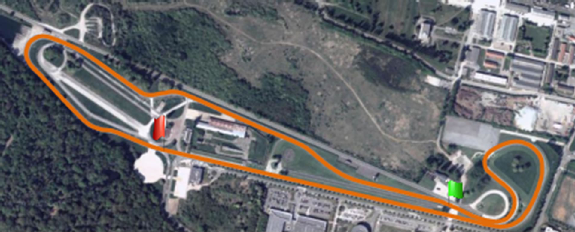
Figure 6. Satory Test Track-Urban Area.
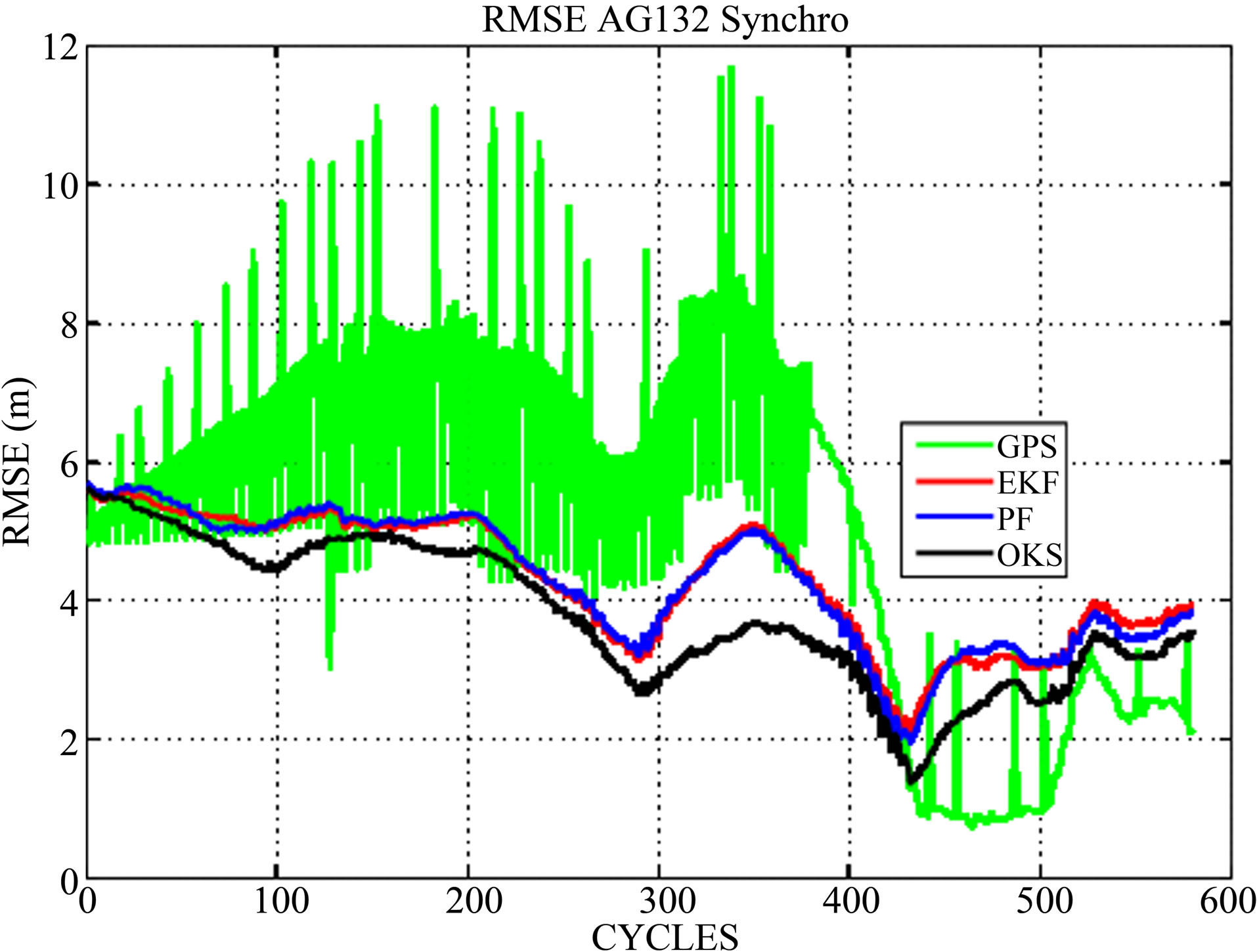
Figure 7. RMSE for AG132 Synchronous data.
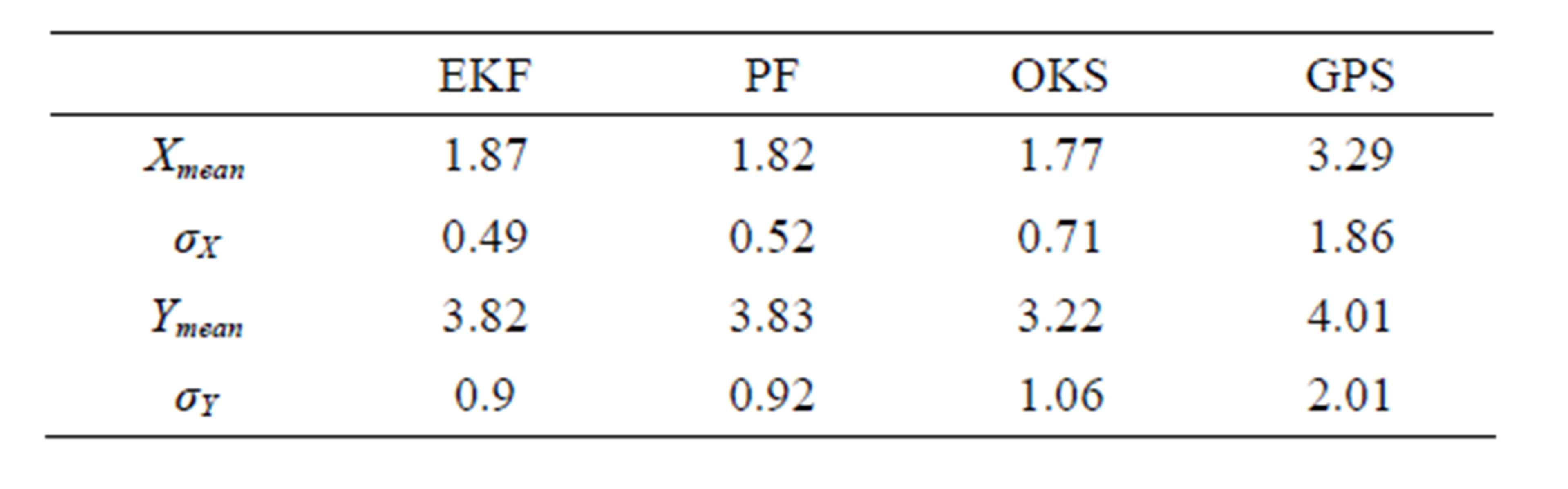
Table 1. Axis Mean Errors and standard deviations (m) for AG132.
clearly the degraded quality of the GPS signal. The filters RMSE given in Figure 7 shows that the EKF filter corrects the errors but remains attracted by the biased GPS corrective data. The three filters, for this test, have quite similar behaviors. The PF performs nearly the same localization as the EKF while the OKS outperforms the two others making use of the cooperative and reactive aspects. To achieve such an accurate positioning, the OKS gives a set of adequate likelihood values to its estimation at each time step. Table 1 gives the axial mean errors and standard deviations in positioning for the GPS data, the EKF, PF and OKS filters. These results confirm the OKS accuracy and robustness to strong noises and bias. These axial errors bounds are also given to show the filters errors ranges. According to the axial means errors, the OKS is then approximately 11% more accurate than the EKF and the PF along this entire first test. Also according to the axial standard deviations, the OKS is 9% less sensitive than the EKF and PF filters.
The capability of the OKS filter to merge information coming from both the prediction and the correction stages using an adapted weighting (fitness) mechanism (taking into account their respective effect) allows to get a better estimation of the vehicle positioning. However, this capacity, which can be a quasi-non consideration of correction data due to their noise, seems to hide a divergence of the filter. To ensure the integrity of our filter, we decided to carry out further tests. In order to test the quality and the performances of the OKS approach in urban driving situation, a GPS disturbance and degradation have been generated. This degradation is similar to the effect of the GPS signal multi-refection.
The two following tests are done on real collected asynchronous AG132 GPS data. The first one will be carried out with the original data without any additional noise or degradation. The second one will integrate urban canyon multipaths to the GPS data in order to test the filters reactivity and sensitivity.
The results of the raw asynchronous GPS data test on the Satory test track are shown in Figure 8 and Table 2. The RMSE graphic shows that the OKS still performs a good positioning, also for normal signal conditions. This performance ensures that the OKS can be efficient in plenty scenarios, not only for bad signal or outage situations. From the Table 2 which shows results of axial mean errors and axial standard deviations, we can conclude that for the correct signal conditions test, the OKS is 1% more accurate and 2.4% more reactive than the other filters.
In order to test the performances of our approach in another difficult situation, we carry out a supplementary test on the AG132 asynchronous data. This last test consists in simulating a driving situation on a city with urban
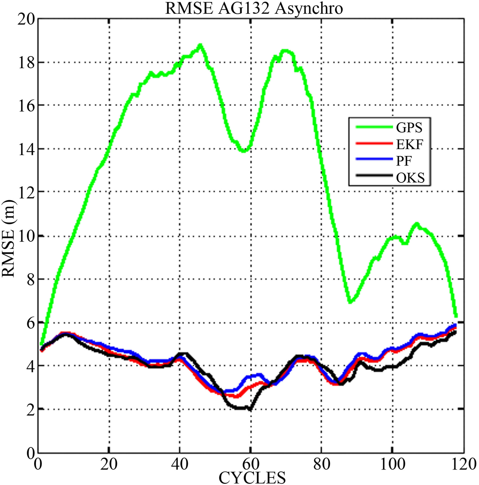
Figure 8. RMSE for AG132 Asynchronous data.
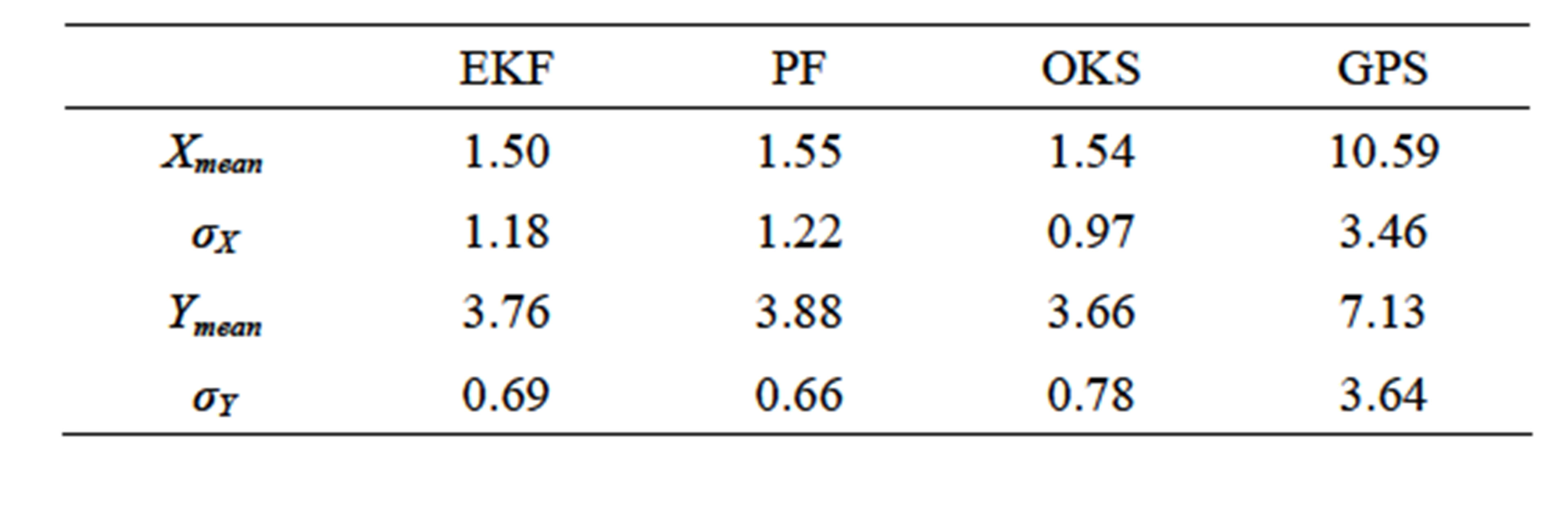
Table 2. Axis Mean Errors and standard deviations (m) for AG132 Asynchronous data.
canyon where almost GPS systems suffer from multipath, multireflexion and outage problems. The multipath errors are simulated and added to the real GPS data used in the previous test. For this test, in Figure 9 the RMSE states that the OKS outcompetes the other approaches especially in signal multireflexion zones. The OKS performs better positioning with a higher accuracy and remain less sensitive to the abrupt positioning changes (peaks in GPS RMSE) than the EKF and PF filters. The results noted in Table 3 prove that the OKS is 10% more precise and 0.9% less sensitive than the other filters. Note that in the peaks zones (multipaths), all the filters are affected but the OKS filter remains more confidents on its estimation and the less sensitive to outliers.
We can see that for all the tests performed the OKS shows better overall results and overtakes EKF general performances in case of noisy GPS data and multipaths.
5. Conclusions
This article highlights a new collaborative technique inspired by Particle Swarm Optimization applied to onroad vehicle localization applications. The advantage of the OKS is an increased robustness in degraded conditions (noises, bias and multireflection). The presented approach outperforms the EKF and the SPF precision and
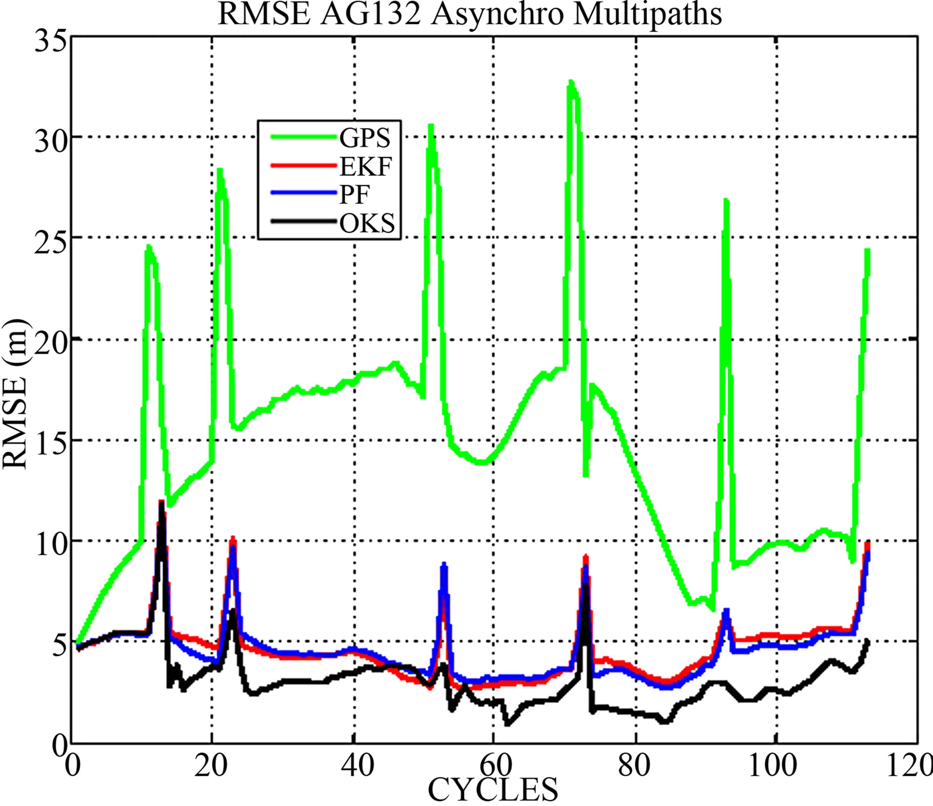
Figure 9. RMSE for AG132 Asynchronous data with multipaths.
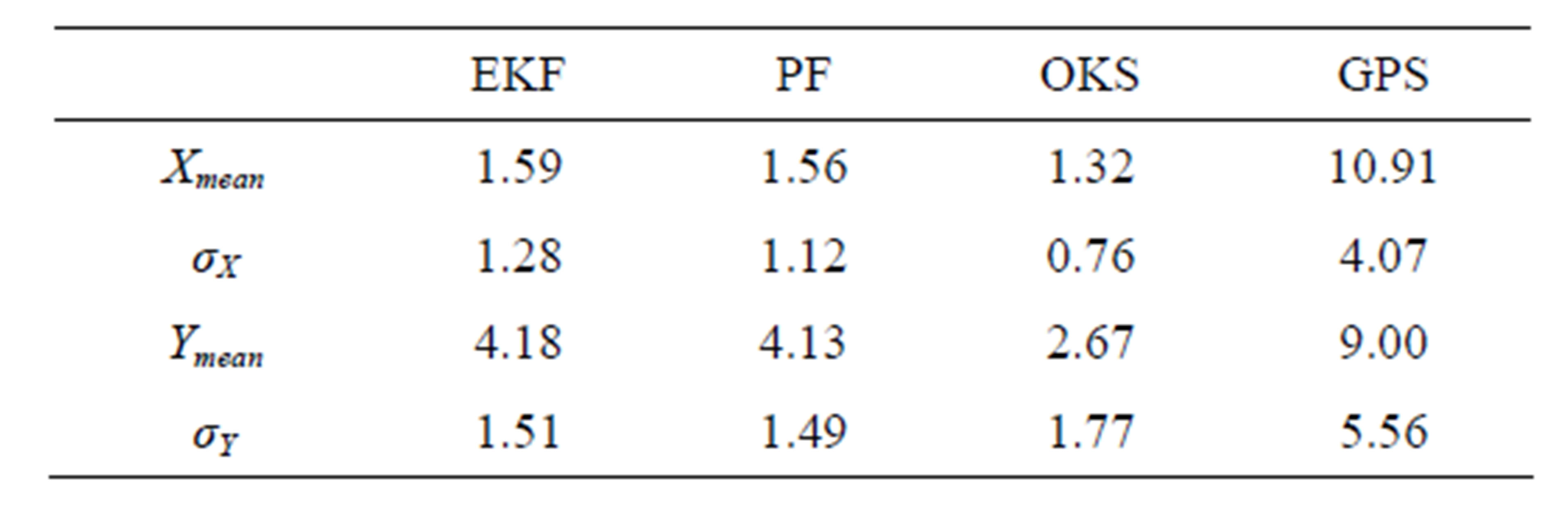
Table 3. Axis Mean Errors and standard deviations (m) for AG132 Asynchronous data with multipaths.
robustness in urban driving scenarios (multipath and signal outage). The OKS reaches these performances making use of an adaptive multi-objective fitness function. In practice, the adaptive fitness function allows the swarm to evolve following high scores. These scores evaluate each particle’s likelihood, balancing between following the current momentum, the prediction or the GPS corrective data, according to their respective assigned or acquired (measured) uncertainties. This compromise makes the OKS method more efficient for on-road vehicle localization applications and especially in urban driving situations.
The EKF method is less time-consuming than the OKS which is similar with the PF when using the same number of particles. Even though the OKS is more computationally complex, the auspicious results given by this filter make it an interesting new localization method. Moreover, the OKS is simple to configure and it has few parameters to be fixed in comparison with some optimization and hybrid localization techniques.
New improving functionalities are studied such as a swarm auto attraction-repulsion mechanism (diversification) preventing the particles premature convergence in a full connected swarm topology. Also intended, a generic fitness function allowing the extension of the system is studied. A future work is to test the OKS performances in diverse driving scenarios such as unusual maneuvers like stop and go, strong braking and acceleration and parking. Also, additional sensors could be interesting to improve the accuracy and the integrity of the OKS approach. A new evolution function with no parameters, no random terms and including the repulsion mechanism is ongoing.
Finally, new criteria of consistency and integrity will be defined in order to compare the OKS to the IMM approach (Multi-Interaction Models) developed by LIVIC for autonomous vehicle localization applications.
REFERENCES
- J. Godoy, D. Gruyer, A. Lambert and J. Villagra, “Development of a Particle Swarm Algorithm for Vehicle Localization,” IEEE Intelligent Vehicles Symposium, Alcala de Henares, 3-7 June 2012, pp. 1114-1119.
- E. Seignez, A. Lambert and T. Maurin, “Autonomous Parking Carrier for Intelligent Vehicle,” IEEE International Conference on Intelligent Vehicle, Nevada, 6-8 June 2005, pp. 411-416.
- A. Ndjeng, A. Lambert, D. Gruyer and S. Glaser, “Experimental Comparison of Kalman Filters for Vehicle Localization,” IEEE Intelligent Vehicles Symposium, Xi’an, 3-5 June 2009, pp. 441-446.
- P. S. Maybeck, “Stochastic Models, Estimation and Control,” Academic Press, New York, 1982.
- F. L. Lewis, “Optimal Estimation: With an Introduction to Stochastic Control Theory,” John Wiley & Sons, New York, 1986.
- R. E. Kalman, “A New Approach to Linear Filtering and Prediction System,” Transactions of the ASME-Journal of Basic Engineering, Vol. 82, 1960, pp. 35-45.
- B. Mourllion, D. Gruyer, A. Lambert and S. Glaser, “Kalman Filters Comparison for Vehicle Localization Data Alignment,” IEEE/RSJ International Conference on Advanced Robotics, Seattle, 18-20 July 2005, pp. 178-185.
- J. Ali and M. R. Ullah Baig Mirza, “Performance Comparison among Some Nonlinear Filters for a Low Cost Sins/Gps Integrated Solution,” Nonlinear Dynamics, Vol. 61, No. 3, 2010, pp. 491-502.
- L. Bazzani, D. Bloisi and V. Murino, “A Comparison of Multi Hypothesis Kalman Filter and Particle Filter for Multi-Target Tracking,” Performance Evaluation of Tracking and Surveillance Workshop at CVPR, Miami, 25 June 2009, pp. 47-54.
- J. Laneurit, C. Blanc, R. Chapuis and L. Trassoudaine, “Multisensorial Data Fusion for Global Vehicle and Obstacles Absolute Positioning,” IEEE Intelligent Vehicles Symposium, Columbus, 9-11 June 2003, pp. 138-143.
- J. S. Gutmann, T. Weigel and B. Nebel, “A Fast, Accurate, and Robust Method for Self-Localization in Polygonal Environments Using Laser Range Finders,” Advanced Robotics Journal, Vol. 14, No. 8, 2001, pp. 651-668. http://dx.doi.org/10.1163/156855301750078720
- I. Abuhadrous, F. Nashashibi and C. Laurgeau, “3-d Land Vehicle Localization: A Real-Time Multi-Sensor Data Fusion Approach Using Rtmaps,” International Conference on Advanced Robotics, University of Coimbra, Portugal, June 30-July 3, 2003, pp. 71-76.
- Y. Shi and R. Eberhart, “A Modified Particle Swarm Optimizer,” IEEE International Conference on Evolutionary Computation, Anchorage, 4-9 May 1998, pp. 69-73.
- M. Reyes-Sierra and C. A. C. Coello, “Multi-Objective Particle Swarm Optimizers: A Survey of the State-of-theArt,” International Journal of Computational Intelligence Research, Vol. 2, No. 3, 2006, pp. 287-308.
- C. A. Coello and M. S. Lechuga, “Mopso: A Proposal for Multiple Objective Particle Swarm Optimization,” IEEE Congress on Evolutionary Computation, Vol. 2, 2002, pp. 1051-1056. http://ieeexplore.ieee.org/xpl/abstractCitations.jsp?tp=&arnumber=1004388&url=http%3A%2F%2Fieeexplore.ieee.org%2Fxpls%2Fabs_all.jsp%3Farnumber%3D1004388
- A. Banks, J. Vincent and C. Anyakoha, “A Review of Particle Swarm Optimization. Part i: Background and Development,” Springer Science, Business Media, 2007.
- S. C. Esquivel and C. A. C. Coello, “On the Use of Particle Swarm Optimization with Multimodal Functions,” IEEE Congress on Evolutionary Computation, Canberra, 8-12 December 2003, pp. 1130-1136.
- R. Havangi, M. A. Nekoui and M. Teshnehlab, “A Multi Swarm Particle Filter for Mobile Robot Localization,” International Journal of Computer Science, Vol. 7, No. 3, 2010, pp. 15-22.
- D.-J. Jwo and S.-C. Chang, “Particle Swarm Optimization for gps Navigation Kalman Filter Adaptation,” Aircraft Engineering and Aerospace Technology, Vol. 81, No. 4, 2009, pp. 343-352. http://dx.doi.org/10.1108/00022660910967336
- M. Clerc and J. Kennedy, “The Particle Swarm-Explosion, Stability, and Convergence in a Multidimensional Complex Space,” IEEE Transactions on Evolutionary Computation, Vol. 6, No. 1, 2002, pp. 58-73. http://dx.doi.org/10.1109/4235.985692
- R. A. Krohling, “Gaussian Swarm: A Novel Particle Swarm Optimization Algorithm,” IEEE Conference on Cybernetics and Intelligent Systems, Vol. 1, Singapore, 1-3 December 2004.
- V. D. B. Frans, “An Analysis of Particle Swarm Optimizers,” Ph.D. Dissertation, University of Pretoria, South Africa, 2002.
- R. E. Xiaohui Hu and Y. H. Shi, “Recent Advances in Particle Swarm,” Congress on Evolutionary Computation, Vol. 1, Portland, 20-23 June 2004.
- J. D. Hol, T. B. Schön and F. Gustafsson, “On Resampling Algorithms for Particle Filters,” Nonlinear Statistical Signal Processing Workshop, Corpus Christi College, Cambridge, 13-15 September 2006.