Positioning
Vol.1 No.1(2010), Article ID:3159,10 pages DOI:10.4236/pos.2010.11002
A New Image Stabilization Model for VehicleNavigation
![]()
College of Computing Sciences, New Jersey Institute of Technology, Newark, USA
Email: shih@njit.edu
Received May 24th, 2010; revised August 24th, 2010; accepted August 28th, 2010
Keywords: Image Stabilization, Image Displacement Compensation, Vehicle Navigation
ABSTRACT
When a video camera is mounted on a vehicle’s frame, it experiences the same ride as a passenger and is subject to vertical displacement as the vehicle hits bumps on the road. This results in a captured video that may be difficult to watch because the bumps are transferred to the recorded video. This paper presents a new image stabilization model for vehicle navigation that can remove the effect of vertical vehicular motion due to road bumps. It uses a wheel sensor that monitors the wheel’s reaction with respect to road disturbances prior to the vehicle’s suspension system. This model employs an inexpensive sensor and control circuitry. The vehicle’s suspension system, bumpy road, and the compensation control system are modeled analytically. Experimental results show that the proposed model works successfully. It can eliminate 10 cm of drift and results in only 1 cm disturbance at the onset and the end of bumps.
1. Introduction
Vehicular imaging systems are common in police vehicles, trucking and transportation systems, rail cars, and buses. Such systems are typically mounted on the vehicle’s frame or a component of the vehicle attached to the frame (e.g. a dashboard), inheriting the ride from the vehicle’s suspension system which protects the frame and passengers. The inspection of videos captured from vehicles is typically nauseating because of the constant jittery motion that is transferred from road perturbations, dampened by the vehicles suspension, and then transferred to the camera. To remedy this problem, three primary methods are usually employed: feature registration, electro-mechanical stabilization, and optical stabilization. Each approach has own advantages and disadvantages that are briefly introduced below.
A common method of image stabilization is feature registration. Brooks [1], Liang et al. [2], and Broggi et al. [3] used feature extraction to lock on a portion of an image in a frame and then employed correction transforms to attempt alignment of the locked target in subsequent frames. This approach is quite computationally intensive, so it limits its real-time applicability. A typical approach identifies a natural horizon or in some cases the lines on a road as a reference to adjust subsequent frames. Since each frame needs to be thoroughly analyzed to identify the reference object and in some cases to determine what to do when there are gaps or missing references, much processing is required for each frame.
A second approach is electro-mechanical stabilization, which employs inertial systems or gyroscopes to detect variations in movement and make corrections to the lens group or imaging plane [4]. Recent advances based on Micro-Electro-Mechanical Systems (MEMS) technology allow gyroscopes to be integrated into Application-Specific Integrated Circuits (ASICs) [5]. The gyroscope measures displacements that are sent to an electronic image stabilization system to perform corrections. The inertial changes can be measured accurately and filtered out, and the appropriate compensation can be made to adjust the image frame. As the price for integrated gyros continues to fall, this approach becomes more favorable nowadays.
Finally, the optical stabilization approach manages a group of lenses in the imaging equipment to compensate for vibration or slow moving disturbances [6-20]. It does not act as quickly as the frame registration or electro-mechanical solutions due to its mechanical compensation.
This paper describes a new image stabilization model for vehicle navigation that can remove the effect of vertical vehicular motion due to road bumps. It uses a wheel sensor that monitors the wheel’s reaction with respect to road disturbances prior to the vehicle’s suspension system. This model employs an inexpensive sensor and control circuitry. The paper is organized as follows. We present the analytical model of the baseline system in Section 2. The analytical model of the electronically stabilized system and experimental results are described in Section 3. Conclusions are drawn in Section 4.
2. Analytical Model of the Baseline System
In this section, we describe a vehicle with an ordinary camera mounted to the vehicle’s frame, which demonstrates a baseline of a typical image viewing experience and the problems occurred. Figure 1 shows a model of a baseline vehicle without electronic camera stabilization. The sensor is in a front wheel assembly, and the camera may be mounted at the head of the vehicle. The schema shows a logical view of the road, wheel, suspension system, and camera assembly. The wheel is modeled as a spring ( ), and the suspension system is modeled as a spring (
 ) and damper (
 ) [11]. The imaging subsystem has a rigid mount to the vehicle’s frame, and thus experiences the same response to road conditions as the vehicle frame does. Collectively, this model of springs and dampers allows one to create a control system model that can describe the behavior of the vehicle’s response to varying road conditions. The force of the ground is labeled as fg(t). The displacements of the road, wheel, and vehicle frame are denoted as Yr, Yw, and Yv, respectively. Each of these displacements is assumed to be 0- valued at the initial condition of t0.
In order to determine the vehicle’s response, the parameters of the model are required. The vehicle data used for the springs and damper in this paper are adapted from [11] as an example of real parameters. These model parameters are itemized in Table 1, where  and
and  denote the spring rates of the suspension and tire respectively,
 and
and denote the sprung and unsprung masses of the vehicle and wheel respectively, and
 denotes the damper rate of the suspension spring. The suspension parameters are well known by vehicle designers. By using the logical model and representative data, we can create an analytical model.
2.1. Analytical Model
Let ,
,  and
and  denote the vertical displacements of the road, wheel, and vehicle from their initial reference positions, respectively. When the vehicle is at rest, these values are assumed to be 0. We can derive the motion equations using Newton’s second law as:
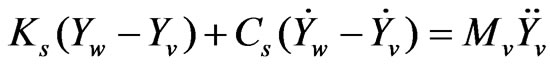 (1)
(1)
 (2)
(2)
Note that the single and double dot notations denote first and second derivatives with respect to time,
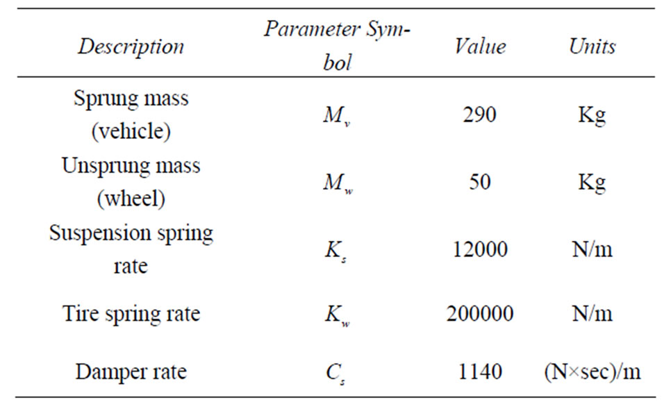
Table 1. Model parameters.

Figure 1. Model of a baseline vehicle without electronic camera stabilization.
respectively. The first derivative of any displacement  is its velocity, while the second derivative
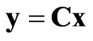
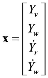
  is its acceleration. These equations can be mapped to the socalled state-space form for this particular problem. The following state-space representation is modified from [12] and is implemented in MATLAB™. Let the variable u denote the input vector, and let y denote the output vector. We have
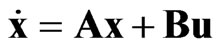 ,
, (3)
(3)
where
 ,
, 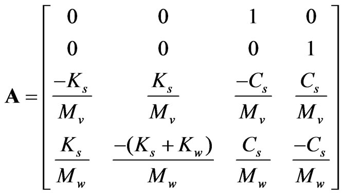
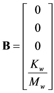 ,
,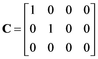 .
.
2.2 Behavior of the Uncompensated System
The vehicle imaging system will share the same ride with the driver. It is subject to the vehicle’s response of the suspension system that can be modeled as a low-pass filter of the bumps in the road as smoothed out by the suspension system. This is referred to as an open-loop system because there is no feedback to the imaging system. For simplicity, we model a bump in the road as a rectangular pulse, which is a 10 cm high disturbance that the vehicle rolls over for approximately 1 second. The vehicle response to this bump and the effect on the image recording are analyzed.
We multiply the B matrix by 0.1 since B is the coefficient for the unit step function u in Equation (3). The step response can be obtained using the MATLAB™ step( ) function. To obtain the response to the whole bump (entering and leaving), the MATLAB™ lsim( ) function from the Control System Toolbox is used. In this case, the resulting response of a 1 second wide bump starting at 0.2 seconds is shown in Figure 2.
The graph in Figure 2 shows the bump (dotted line), the response of the wheel ( ), and the response of the vehicular frame (
 ) which is the representative of the camera’s response to the bump over time. The y-axis is the displacement in meters. It can be seen that the wheel response is quick and abrupt. The vehicular frame benefits from the additional spring and damper system of the car’s shock absorbers. It shows a smoother, more delayed response and produces the overshoot and undershoot of the frame. It actually ascends higher than the bump and

Figure 2. Response of a 1 second wide bump starting at 0.2 seconds.
then dips back down to a negative displacement for a short while. Note that different parameters for the springs and the damper (shock absorber) will result in different responses of the car.
2.3. Image Viewing Experience of the Open-Loop System
We apply the aforementioned vehicle frame response to the imaging plane using the displacements of the  curve as offsets from a representative image. Figure 3 shows the reference scene for the effect of vehicle bounce. It is observed that the white line appears on the road and it is smooth and linear. This is visibly distorted by the bump.
Next, the response of a 1 second wide bump starting at 0.2 seconds,  , shown in Figure 2, is mapped to the image of the viewer’s experience. This is done by sweeping through the image left-to-right and a vertical row at a time. Each vertical row represents a time interval. Each vertical row of pixels is viewed as a point in time or a frame of a video sequence. By taking the signal
  and scale it to displace the row of image pixels over time, the effect of a video is created.
From the vehicle’s perspective, a comfortable ride for the user and a safe ride for the vehicle are paramount. From the camera’s perspective, we wish to completely flatten out this response, so the view is level. From Figure 4, the representative image viewed on the display of an unstabilized imaging system results in a view that has both large disturbances and a lasting effect because of the damping response of the suspension. It is the effect to be eliminated with electronic image stabilization.
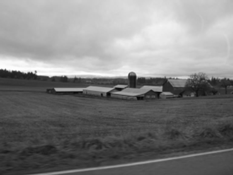
Figure 3. The reference scene for the effect of vehicle bounce.
3. Analytical Model of the Electronically Stabilized System
In this section, we present the analytical model of the electronically stabilized system. Some suspension systems are characterized as an active suspension, in which the damper Cs is an active element whose stiffness is adjusted by an active control system [10]. The closedloop nature of the system is resulted from feedback and control in the electrical form, feeding the imaging subsystem. Thus, the closed-loop control is for the image display platform, not for the vehicle’s ride. This closedloop attribute allows the imaging subsystem to monitor the response of the wheel on the road and make adjustments that coincide with the vehicle’s frame which holds the imaging subsystem [13-16].
Figure 1 is modified by a sensor device attached to the vehicle’s wheel assembly as shown in Figure 4. The sensor relays an analog electrical voltage signal that
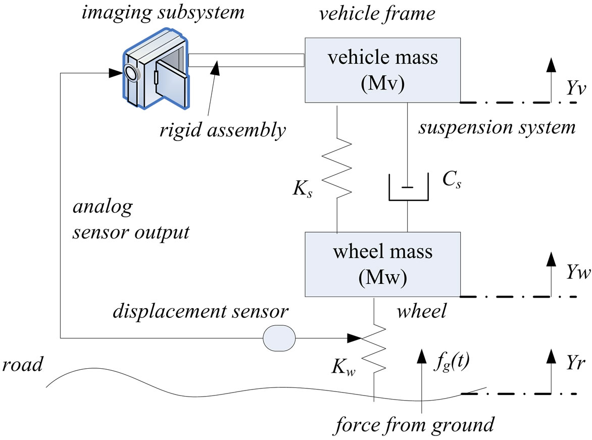
Figure 4. Model of image stabilizer physical assembly.
provides a linear measurement of the displacement of the sensor’s internal piston. This could be a low-friction potentiometer assembly. As part of the imaging subsystem, the sensor input is digitized to provide a real-time feed of displacement data sampled at the rate of 100 samples per second.
With the addition of a sensor and its output, we can further elaborate the diagram to show the logical view of the model which includes the active controller for image stabilization. This new model is depicted in Figure 5, which shows that a video camera assembly with a large vertical aspect ratio is used to gain an extra vertical displacement margin. This is necessary because the compensator will make use of this slack to realign the picture.
If the extra image from this margin is available, it helps remove blank information from being in the compensated frames. The output of the camera is fed to an image processing block, called a displacement compensation control function G(z). This block receives the wheel sensor’s displacement data,  as an input to the block. The processing function in the G(z) block is applied to compensate for the response that the frame is about to experience as a result of a bump on the road. After computation, it arrives at a vertical displacement compensation by which the received frame needs to be adjusted to give appearance of a smooth video. This is simply a re-registration of the vertical offset of the frame. The displacement margins are beneficial since the image re-registration within the displacement margin allows an image to completely cover the resulting frame instead of a portion of it being blank where no image is captured. The resulting image frames are sent to an appropriate recording device.
The electronic stabilization model aims to determine the appropriate control function G(z), so the video captured by the imaging subsystem can generate reasonably good images. Note that the whole frame is displaced by  as the vehicle experiences bumps, but G(z) will receive an earlier response directly from the wheel. If the processing is fast enough, then G(z) can issue a displacement compensation offset to the electronic imager to adjust the frame rendered offset through re-registration in real-time as the vehicle frame experiences the response from the suspension system. This is important because since we wish to view the video being captured as events happen. This approach allows real-time monitoring.
3.1. Deriving the Stabilization Control Function
The next step is determining the control filter G(z), such that its processing of  summed with
  will result in a relatively smooth output R(t). This is illustrated in Figure 6, where G1(z), G2(z), and G(z) are transfer functions. G1(z) and G2(z) are derived in the

Figure 5. Logical model of the system with the electronic image stabilizer.
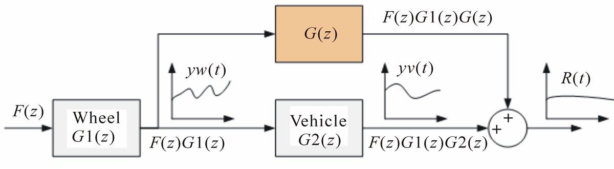
Figure 6. Control theoretical view of the electronic image stabilizer.
continuous time domain, and their state-space representation is given. They are processed in the discrete timedomain since the output  is sampled by the wheel sensor and since G(z) performs digital image processing tasks.
By using MATLAB c2d( ) function, the continuous time state-space representation is converted to a discrete time model given the sample rate. By defining a 0.01 second (100 Hz) sample rate, the resulting transfer functions for G1(z) and G2(z) can be obtained as:
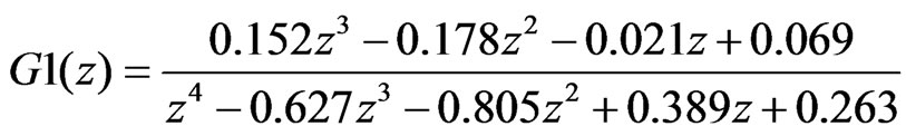 (4)
(4)
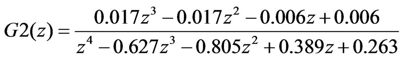 (5)
(5)
The output response of G1(z) is simply the input F(z) multiplied by the transfer function G1(z) when working in the z domain. Similarly, the output response of G2(z) is the response of F(z)G1(z) multiplied by G2(z). Lastly, the response of the unknown transfer function G(z) is also derived in the same manner.
We intend to achieve a smooth output at R(t). By observing that the result of the summation junction is required to be 0, we can obtain the following relation:
 (6)
(6)
By solving for G(z), we obtain
 (7)
(7)
The only way to cancel the response of G2(z) is through an identical negative value. If taking the response F(z)G1(z) from the wheel and applying G2(z) through processing, we can use this response to compensate for the vehicle’s response, in effect to predict the vehicles response before it occurs. It produces real-time processing for imaging stabilization.
3.2. Calculation of the Compensator G(z)
In this section the digitized sampling of  is illustrated and applied to the G(z) transfer function to determine its response. This information is then used to compare the G(z) and G2(z) paths for similarity. Figure 7 shows the sampled signal from the wheel,
 , which is a result of the ground force F(z) multiplied by the wheel transfer function G1(z).
By using the sample rate of 100 Hz, it is necessary to sample the relatively high-frequency response of the wheel as compared to the frame that is damped. Figure 8 shows a small portion of Figure 7 which is zoomed in. It can be seen that we have a sufficiently high sample rate to ensure a good quality representation of the input image since the Nyquist’s theorem suggests the sampling rate to be at least two times the highest frequency component.
Next, we show in Figure 9 the continuous time response from the vehicle, , and the sampled signal from Figure 7,
  , superimposed together to check how close they are. It can be seen that the compensator transfer function successfully predicts the response of the vehicle. When the signal is subtracted, we expect much of the disturbance to be removed. The minor differences may be attributed to the sampling points, which are asynchronous (but periodic) to the continuous time image. The small differences in time may be the source of error.
With the predicted compensation from the G(z) transfer function, we can re-register each image frame with a negative offset equal to the response of G(z). This image processing function of a y-axis offset is trivial. The field of view is buffered with a sufficient displacement margin to allow the frame to be re-registered without losing any portion of the image. The registration and margin
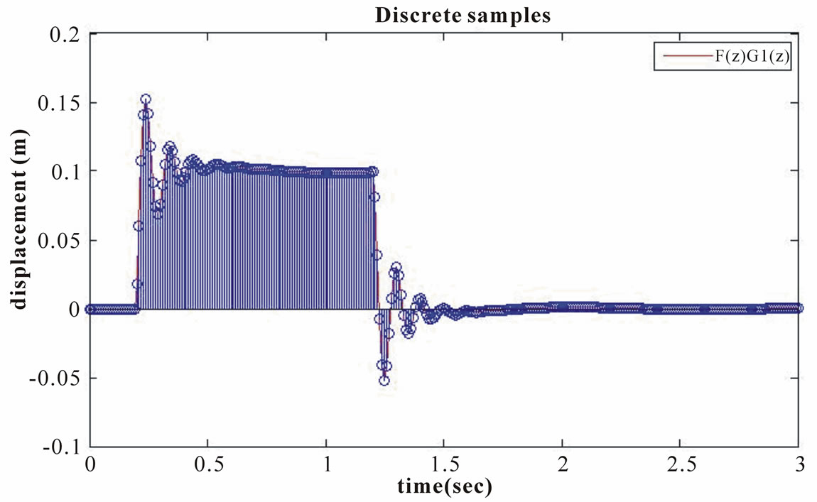
Figure 7. Sampled signal response of F(z)G1(z), .
.
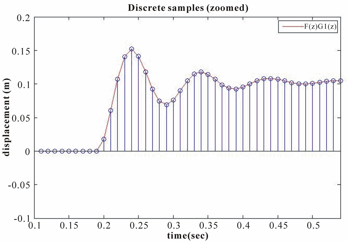

Figure 9. Comparison of vehicle frame’s response to the compensator’s response.
concepts are illustrated in Figure 10. In practice, these margins are available by a larger field of view than normally shown on the display, or perhaps by the image cropped to a smaller size than the regular field of view. In either case, the margin is gained.
3.3. Viewing Experience with the Electronically Stabilized Imaging System
Finally, we show the result of the summation of the vehicle’s response and the negative of the compensated response. The final response, R(t), also the resulting error of the system, is shown in Figure 11. It is impossible to perform a perfect correction, but through the proposed method, the error seems to be roughly about 1 cm. It seems to appear both at the onset of the disturbance and the relief of the disturbance.
The viewing image can be obtained by displacing the image columns by the amount in the scaled signal R(t). For the image processor, it is the output of G(z) that is used as a negative displacement for image registration. It is in effect the same as the final displacement offset errors that one can see in the resulting image sequence. This effect is shown in Figure 12, where the reference signal is superimposed as a dashed line for comparison. It is observed that the image quality using the proposed electronic image stabilization model has been significantly improved. The resulting image, while still experiencing a slight effect of the bump, has been largely smoothed out.
3.4. Experimental Results
Experimental results show that the disturbance causes
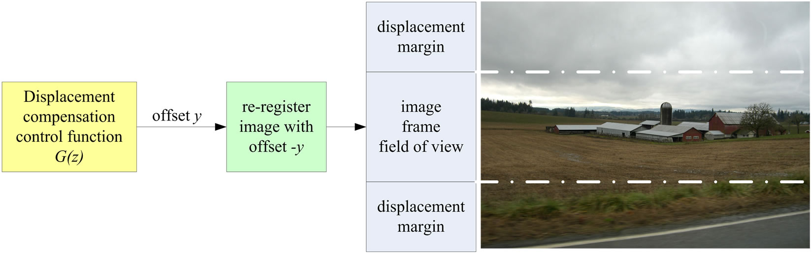
Figure 10. Final response, R(t), is also the resulting error of the system.
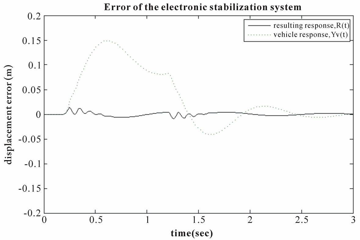
Figure 11. Final response, R(t), is also the resulting error of the system.
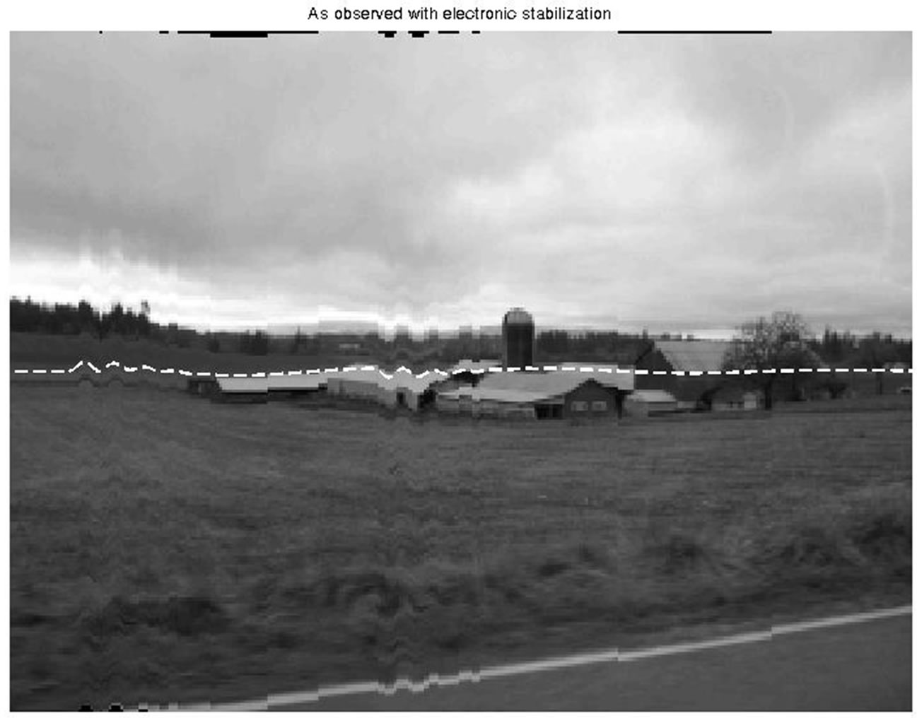
Figure 12. Simulated bump experience of the compensated system.
about 6 pixels of error over a frame of 301 × 226 pixels by using the proposed method. This error range is about 2.6% of the frame’s vertical size (226 pixels). The results are better than the image stabilization method by Brooks [1], which stabilized the image to within 10-20 pixels of displacement error, and the method by Khajavi and Abdollahi [11], which produced the error in the range of 3.9 to 7.8%.
The goal of Liang et al. [2] is similar to ours; however, they used road lane markings for the reference to stabilize the video. Its performance seems good, but its measure of accuracy is the angular error. Because their approach is highly dependent on the visibility and availability of road lane markings, it is not practical for a general purpose system.
Broggi et al. [3] presented an approach of employing image processing algorithms. This computationallyintensive approach performs a series of digital filters to provide stabilization. Their results generated a compensated pixel variability of approximately 4 pixels when approximately 45 pixels of distortion were introduced, which is an error of 8.9%. They also showed that when an infrared video imaging system is used, an error of 5.4% is achieved.
4. Conclusions
We have developed an electronic image stabilization model which can receive an early indication of the ride since the vehicle frame is delayed slightly by the response of the spring and damper in the vehicle’s suspension system. A control system of the road, vehicle, and the compensating transfer function are modeled. The compensating transfer function is determined analytically based on the modeled response of the vehicle’s suspension system. A simple sensor arrangement feeds the compensator real-time data from the wheel assembly and processes it through the compensator’s transfer function. This information is then subtracted from the image plane through simple vertical image registration, thus removing (compensating) the vehicle’s response to which the camera is attached.
REFERENCES
- A. Brooks, “Real-Time Digital Image Stabilization,” Electrical Engineering Department, Northwestern University, Evanston, Illinois, 2003.
- Y. Liang, H. Tyan, S. Chang, H. Liao and S. Chen, “Video Stabilization for a Camcorder Mounted a Moving Vehicle,” IEEE Transactions on Vehicular Technology, Vol. 53, No. 6, 2004, pp. 1636-1648.
- A. Broggi, P. Grisleri, T. Graf and M. Meinecke, “A Software Video Stabilization System for Automotive Oriented Applications,” Proceedings of IEEE Conference on Vehicular Technology, Dallas, TX, 2005, pp. 2760-2764.
- F. Panerai, G. Metta and G. Sandini, “Adaptive Image Stabilization: A Need for Vision-Based Active Robotic Agents,” Proceedings of Conference on Simulation of Adaptive Behavior, Paris, France, 2000.
- D. Sachs, S. Nasiri and D. Goehl, “Image Stabilization Technology Overview,” InvenSense Whitepaper, 2006.
- K. Sato, S. Ishizuka, A. Nikami and M. Sato, “Control Techniques for Optical Image Stabilizing System,” IEEE Transactions on Consumer Electronics, Vol. 39, No. 3, 1993, pp. 461-466.
- J. S. Jin, Z. Zhu and G. Xu, “A Stable Vision System for Moving Vehicles,” IEEE Transactions on Intelligent Transportation Systems, Vol. 1, No. 1, 2000, pp. 32-39.
- Z. Zhu, “Full View Spatio-Temporal Visual Navigation—Imaging, Modeling and Representation of Real Scenes,” China Higher Education Press, China, 2001.
- B. Chan and C. Sandu, “A Ray Tracing Approach to Simulation and Evaluation of a Real-Time Quarter Car Model with Semi-Active Suspension System Using Matlab,” Proceedings of Design Engineering Technical Conference, Chicago, Illinois, 2003, pp. 2129-2134.
- N. Nise, “Control Systems Engineering,” 4th Edition, Wiley, Hoboken, New Jersey, 2004.
- M. Khajavi and V. Abdollahi, “Comparison between Optimized Passive Vehicle Suspension System and Semi Active Fuzzy Logic Controlled Suspension System Regarding Ride and Handling,” Transactions on Engineering, Computing and Technology, Vol. 19, 2007, pp. 57-61.
- W. C. Messner, D. Tilbury and W. Messner, “Control Tutorials for MATLAB and Simulink: A Web-Based Approach,” Prentice Hall, Englewood Cliffs, New Jersey, 1998.
- C. Morimoto and R. Chellappa, “Fast Electronic Digital Image Stabilization for Off-Road Navigation,” Real-Time Imaging, Vol. 2, No. 5, 1996, pp. 285-296.
- Z. Duric, and A. Rosenfeld, “Image sequence Stabilization in Real Time,” Real-Time Imaging, Vol. 2, No. 5, 1996, pp. 271-284.
- M. A. Turk, D. G. Morgenthaler, K. D. Gremban and M. Marra, “VITS—A Vision System for Autonomous Land Vehicle Navigation,” IEEE Transactions on Pattern Analysis and Machine Intelligence, Vol. 10, No. 3, 1988, pp. 342-361.
- S. B. Balakirsky and R. Chellappa, “Performance Characterization of Image Stabilization Algorithms,” Proceedings of International Conference of Image Processing, Lausanne, Switzerland, 1996, pp. 413-416.
- Z. Durica, R. Goldenbergc, E. Rivlina and A. Rosenfeld, “Estimating Relative Vehicle Motions in Traffic Scenes,” Pattern Recognition, Vol. 35, No. 6, 2002, pp. 1339-1353.
- A. Cretual and F. Chaumette, “Dynamic Stabilization of a Pan and Tilt Camera for Submarine Image Visualization,” Computer Vision and Image Understanding, Vol. 79, No. 1, 2000, pp. 47-65.
- Z. Duric, E. Rivlin and A. Rosenfeld, “Qualitative Description of Camera Motion from Histograms of Normal Flow,” Proceedings of International Conference of Pattern Recognition, Barcelona, Spain, Vol. 3, 2000, pp. 194-198.
- S. Sugimoto, H. Tateda, H. Takahashi and M. Okutomi, “Obstacle Detection Using Millimeter-Wave Radar and its Visualization on Image Sequence,” Proceedings of International Conference of Pattern Recognition, Cambridge, UK, Vol. 3, 2004, pp. 342-345.