Natural Science
Vol.4 No.10(2012), Article ID:23917,15 pages DOI:10.4236/ns.2012.410100
Vegetation regrowth trends in post forest fire ecosystems across North America from 2000 to 2010
![]()
1NASA Ames Research Center, Moffett Field, USA; *Corresponding Author: chris.potter@nasa.gov
2California State University Monterey Bay, Seaside, USA
Received 29 August 2012; revised 30 September 2012; accepted 15 October 2012
Keywords: MODIS EVI; Post-Fire Forest; Regrowth; Climate Change; North America
ABSTRACT
The goal of this study was to determine whether climate has affected vegetation regrowth over the past decade (2000 to 2010) in post-fire forest ecosystems of the United States and Canada. Our methodology detected trends in the monthly MODerate resolution Imaging Spectroradiometer (MODIS) Enhanced Vegetation Index (EVI) timeseries within forest areas that burned between 1984 and 1999. The trends in summed growing season EVI (composited to 8 km spatial resolution) within all burned area perimeters showed that nearly 1.6% post-fire forest area declined in vegetation greenness cover significantly (p < 0.05) over the past decade. Nearly 62% of all post-fire forest area showed a non significant EVI regrowth trend from 2000 to 2010. Regression results detected numerous significantly negative trend pixels in post-fire areas from 1994-1999 to indicate that forest regrowth has not yet occurred to any measurable level in many recent wildfire areas across the continent. We found several noteworthy relationships between annual temperature and precipitation patterns and negative post-fire forest EVI trends across North America. Change patterns in the climate moisture index (CMI), growing degree days (GDD), and the standardized precipitation index (SPI) were associated with post-fire forest EVI trends. We conclude that temperature warming-induced change and variability of precipitation at local and regional scales may have altered the trends of large post-fire forest regrowth and could be impacting the resilience of post-fire forest ecosystems in North America.
1. INTRODUCTION
In the first several decades following a stand-replacing wildfire, forest ecosystems typically follow a trend of increasing green vegetation cover and productivity [1-4]. Various environment and climate factors determine the specific rate of the post-fire vegetation recovery, including geographic location, elevation, and extreme weather events [5]. Localized variations in weather conditions (precipitation, temperature, or solar radiation) may cause fine-scale (on the order of a few kilometers) heterogeneity the forest recovery trends within individual wildfire boundaries.
Evidence from historical data sets suggests that 20th Century climate warming may have been associated with increased rates of forest disturbance [6,7]. The increasing frequency and intensity of wildfire disturbance produces potential feedbacks on climate through changes in albedo, forest succession, and carbon sequestration during regrowth [8-10]. The trend (positive or negative) in post-fire forest regrowth rates is of interest to both scientists and land managers who are together assessing the sensitivity of natural forest ecosystems to climate change.
Post-fire forest regrowth has increasingly drawn interest from the climate change and global warming research communities. Previous studies have focused mainly on variations in recovery rates of biogeochemical cycling and carbon sequestration [11-14] analyzed the seasonal and inter-annual variations of post-fire forest cover by using AVHRR-NDVI (Advanced Very High Resolution Radiometer-Normalized Difference Vegetation Index) time-series across boreal North America. They noted that temporal anomalies of NDVI were associated with vegetation compositional changes consistent with early successional plant species and susceptibility to drought. [2] utilized a 19-year time-series of AVHRR-NDVI data, focusing on several hundred large fires across the western United States. Their results suggested that the regrowth trends of post-fire forests were influenced by variations in surface temperature and precipitation.
Nonetheless, past climate change impacts on post-fire forest recovery processes are not well-understood. Regenerating forests require decades to reach mature stages and begin to show ecosystem resiliency in biomass production. In this study, we utilized over ten years of the MODerate resolution Imaging Spectroradiometer (MODIS) Enhanced Vegetation Index (EVI) data to examine the relationships between vegetation growth trends and climate factors during post-200 wildfire forest succession. We conducted trend mapping for large wildfire areas across all of North America, and detected break points in the recovery patterns of all forest areas burned since 1984. The results of these analyses for the years 2000 to 2010 were intended to provide a baseline for long-term (>10 years) climate change and forest regrowth studies to come after the year 2010.
2. STUDY AREA AND DATA SOURCES
2.1. Study Area
The time period of interest covered all of North America from 1984 to 2010 (Figure 1). Burned forest areas that we separated into five-year intervals showed an increasing frequency of wildfire since 1984 (Table 1 and Figure 2). The historical data presented here were provided solely to identify MODIS pixels for post-2000 forest regrowth analysis. We can draw no a priori conclusions whatsoever about the potential relationships between climate change and wildfire frequency (from 1984 onward) based on the data presented in Table 1 alone.
2.2. Remote Sensing Datasets
Collection 5 MODIS data sets beginning in the year 2000 were obtained from NASA’s Land Processes Distributed Active Archive Center site [15]. MODIS EVI values were aggregated to 8 km resolution from MOD 13C2 (MODIS/Terra Vegetation Indices) products. MOD 13C2 data are cloud-free spatial composites of the gridded 16-day 1-kilometer MOD13A2 product, and were provided monthly as a level-3 product projected on a 0.05 degree (5600-meter) geographic Climate Modeling Grid (CMG). Cloud-free global coverage was achieved by replacing clouds with the historical MODIS time-series EVI record. MODIS EVI was calculated from red, blue and NIR bands as described by [16].
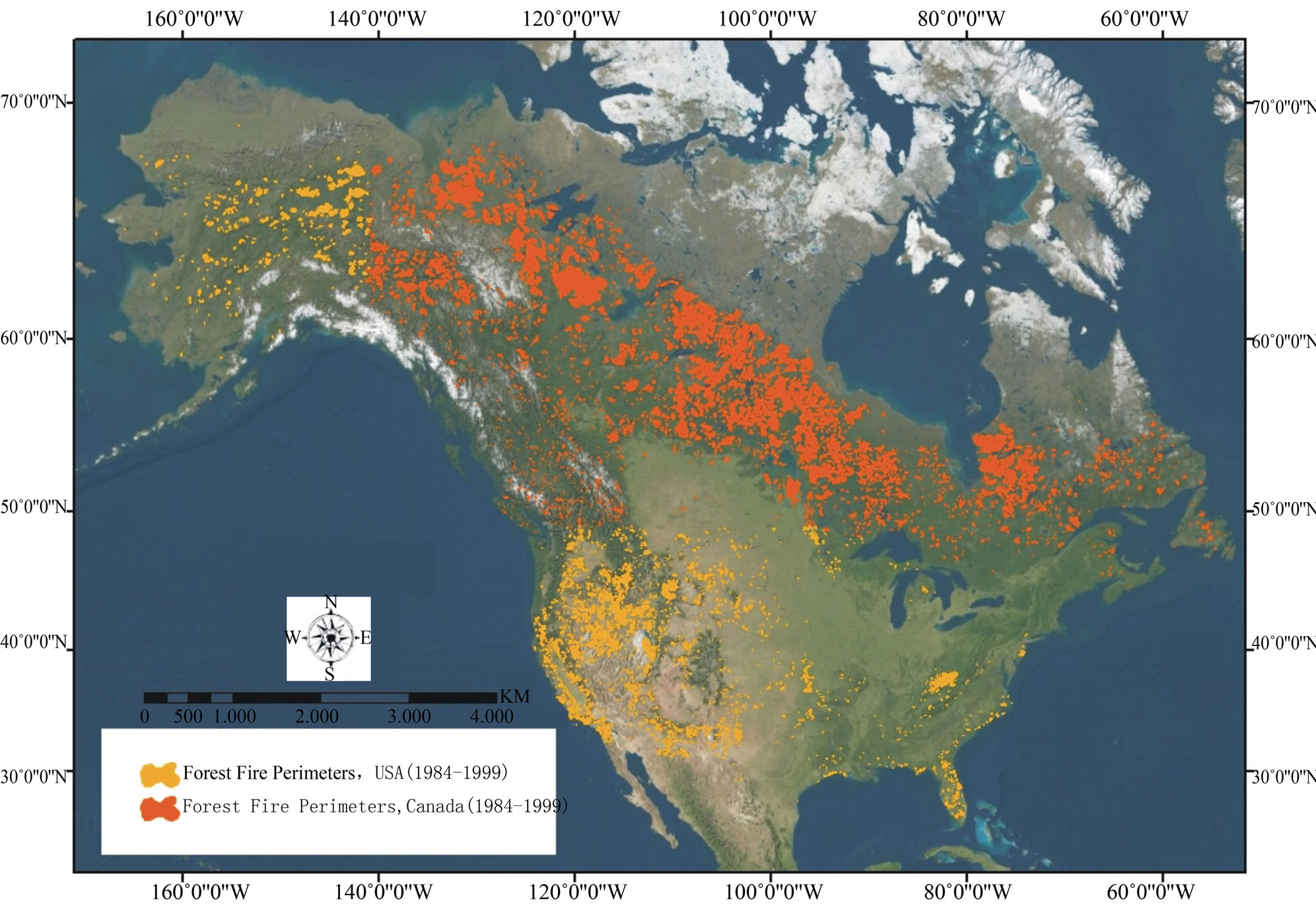
Figure 1. Spatial distribution of forest fire perimeters (1984-1999) across North America. The forest fire polygon data were taken from MTBS (USA) and CNFDB (Canada).
 (a)
(a) (b)
(b)
Figure 2. Wildfire over time in North America. (a) Burned area; (b) Wildfire frequency. Data for this graph were derived from MTBS (USA) and CNFDB (Canada). The curve in plot (a) is fitted using a regression model, and its 95% confidence band is the shaded light blue area.
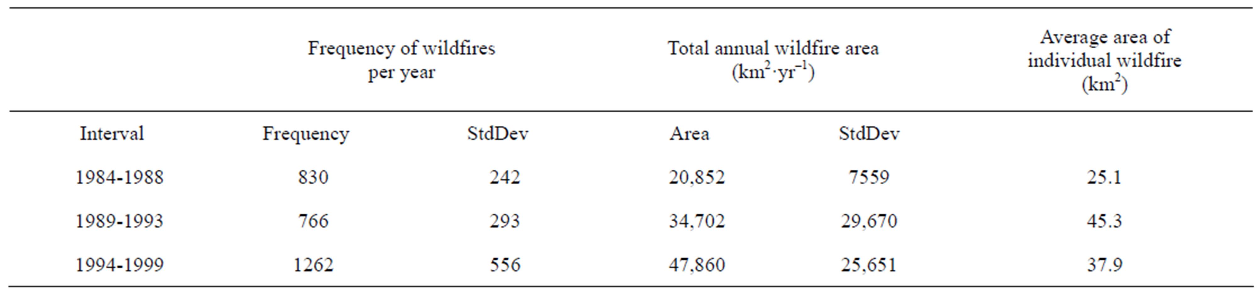
Table 1. Attributes of North American wildfire (1984-1999) that were sampled for post-2000 regrowth analysis.
2.3. Auxillary Datasets
2.3.1. Wildfire Perimeters
A complete North American wildfire history was compiled from two national fire databases, the National Monitoring Trends in Burn Severity (MTBS, USA) and the Canadian National Fire Database (CNFDB).
The MTBS is a multi-year project designed to consistently map the burn severity and perimeters of fires across all lands of the United States for the period spanning 1984 through 2010 [17]. The fire perimeters are vector polygons of the extent of the burned areas, including the continental United States, Alaska, Hawaii and Puerto Rico. The CNFDB point and polygon data are a collection of forest fire locations and fire perimeters as provided by Canadian fire management agencies including provinces, territories, and Parks Canada [18].
Both of the two national wildfire databases were compiled into a consistent data structure and only wildfire areas larger than 64 km2 (corresponding to MODIS 8 km spatial resolution) were used in this study. To control for time since stand-replacing forest disturbance, the database was split into three 5-year intervals (Table 1).
2.3.2. Land Cover Databases
NLCD2001 (National Land Cover Database 2001, USA, [19]) and LCC2000-V (Land Cover, circa 2000- Vector, Canada) were combined to determine the land cover fraction of non-burnable water bodies and bare ground in each 8 km MODIS pixel.
2.3.3. Meteorological Data
We used climate data from National Centers for Environmental Prediction/National Center for Atmospheric Research (NCEP/NCAR) Reanalysis (R1) database, dating back to 1948 [20]. For the purposes of this study, monthly air temperature (2000-2010; mean, maximum, minimum), and monthly total precipitation (PPT, 1980- 2010) were extracted from NCEP R1. Monthly potential evapotranspiration (PET) from global NCEP R1 sources [21] were also prepared for analysis.
Annual climate indexes for each year 2000-2010 were calculated from these monthly meteorological datasets to use as independent explanatory variables for forest recovery trends from wildfire. The climate index selection was based on previous study results from [22], which showed that degree days, annual precipitation totalsand an annual moisture index together can account to 70% - 80% of the geographical variation in the global vegetation seasonal extremes. Selected indexes in this study included: the climate moisture index (CMI, [23]), growing degree days (GDD) base 0˚C, and the standardized precipitation index with time scale of 3 months (SPI, [24]).
The CMI is an aggregate measure of potential water availability imposed solely by climate, which was denfined as: (PPT/PET)-1 if PPT < PET or 1-(PET/PPT) if PPT > PET. The CMI indicator ranges from –1 to +1, with negative values for relatively dry years, and positive values for relatively wet years. GDD is the number of days for which mean monthly temperature was greater than 0˚C. SPI is a probability index that can provide superior representation of abnormal wetness and dryness than the Palmer drought indices. SPI values are positive (or negative) for greater (or lower) than the median precipitation amount. SPI values higher (or lower) than 2.00 (or –2.00) can be considered extreme wet (or dry) events [25]. An extended precipitation history period of 1980 to 2010 was used in this study for SPI calculation, since there is the requirement for fitting a 2-parameter gamma distribution.
3. METHODS
As an overview of our methodology (Figure 3), we developed maps of EVI trends across North America from 2000 to 2010, Forest areas disturbed by wildfires from 1984 to 1999 were separated by five-year age in
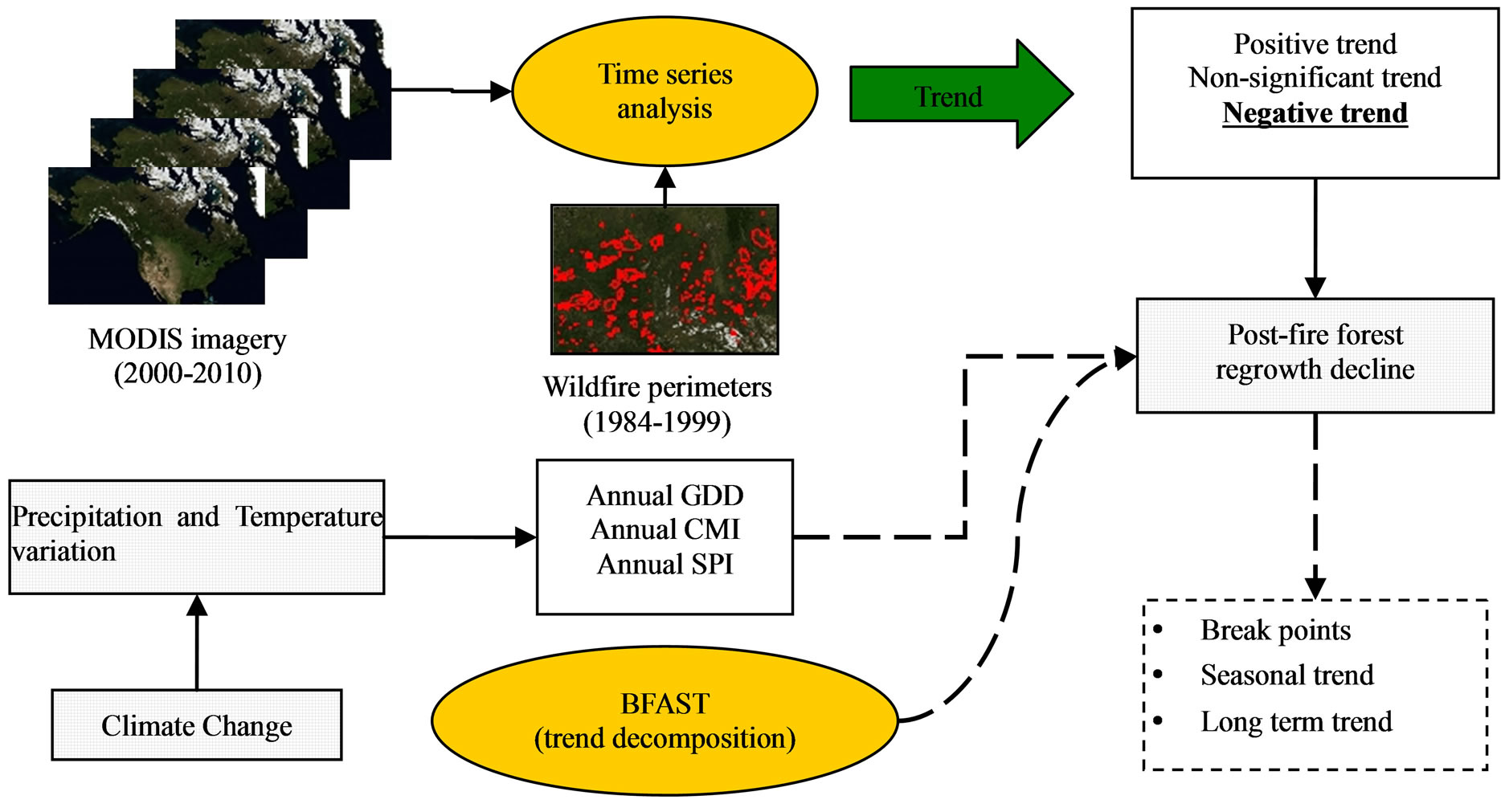
Figure 3. Flow chart of the methodology used to characterize the post-fire forest regrowth trends across North America from 2000 through 2010. Climate data sets are shown in checkered boxed and climate data comparisons with EVI are shown as dashed lines.
tervals. According to the values of the slope and the coefficient of determination (R2) of the EVI regressions, post-fire pixels were classified into three categories, i.e. Positive trend, Negative trend, and Non-significant trend. The “Breaks for Additive Seasonal and Trend” method (BFAST, [26,27]) was further applied to EVI for post-fire trend characterization.
The least squares method was applied to calculate the linear trend line that best fit the EVI data values. We first resampled monthly MOD13C2 EVI data into 8 km areas. The EVI values were then summed across a six-month growing season period (May through September) for each year, 2000-2010. This resulted in a series of annually integrated EVI values representing the variability of vegetation productivity across North America for the past 11 years.
The EVI trend at each pixel was evaluated by regressing the integrated EVI values on time by using the simple linear regression model (Eq.1).
 (1)
(1)
where EVI is the integrated EVI values, Ti is the MODIS data capture year. An ordinary least squares estimate of β (EVI trend slope) and associated R2 were established for each pixel in the research region. The trends of annual climate indexes (CMI, GDD, and SPI) were also generated following the abovementioned method.
Wildfire perimeter databases (MTBS and CNFDB) were used to determine the post-fire forest areas and ages where wildfire occurred over the period of 1984-1999. All 8 km resolution MODIS EVI pixels falling entirely within the wildfire perimeters were defined as 100% post-fire vegetation cover and these were the only pixels included in our analysis.
In order to eliminate the influence from water bodies and bare ground on the results, land cover databases (NLCD2001 and LCC2000-V) with 30 m resolution were used to determine the fraction of non-burnable area in each 8 km pixel. Only pixels covered by burnable vegetation of more than 50% total area were considered burnable pixels and included in our analysis. All non-burnable pixels were masked out and excluded from our analysis dataset.
The post-fire pixels were split into three EVI trend classes for the past decade (2000-2010): 1) Pixels with positive trend, where Slope > 0 and R2 ≥ 0.37 with a 95% level of significance for a two-tailed t-test. 2) Pixels with negative trend, where Slope < 0 and R2 ≥ 0.37. 3) Pixels with non-significant trend (R2 < 0.37, Slope > 0, or Slope < 0).
The BFAST (Breaks for Additive Seasonal and Trend) methodology was next applied for the EVI forest pixels found to belong in the negative trend class. BFAST was proposed by [26,27] for detecting and characterizing abrupt changes within a time series, while also adjusting for regular seasonal cycles. A harmonic seasonal model was implemented in BFAST to account for phenological changes. This methodology required fewer observations and was more robust against noise, compared to traditional principal component analysis (PCA) [28], wavelet decomposition [29], and Fourier analysis.
4. RESULTS
4.1. Post-Fire Regrowth Trends
Both the regression coefficient of determination (R2) and the slope of the linear regression line were retrieved for every MODIS pixel to show the spatial pattern of EVI variation across North America (Figure 4). Positive slope values would likely represent a regenerating vegetation status of the burned forest ecosystem, while negative slope values would likely indicate that vegetation may have slowed in regrowth or started to decline in green cover after disturbance.
A total of 103 post-fire forest locations with signifycant negative EVI trends were found to be scattered across North America, with some clustering of the negative trend class in Alaska and in boreal forest regions of the continental US and Canada (Figure 5). Out of a total of >6500 burned 8 km areas, nearly 1.6% of post-fire pixels from 1984-1999 were detected in the negative EVI trend class whereas 36.6% were detected in the positive trend class, and 61.8% in the non-significant trend class (Table 2). The percentage of pixels in the significant negative EVI trend class increased with the increase of post-fire forest age interval. In contrast, the percentage of pixels with a significant positive EVI trend decreased with the increase of post-fire forest age interval (see arrows in Table 2).
Yearly changes in average slope of growing season EVI over the period 2000-2010 in wildfire areas revealed that green vegetation cover has increased as the time since fire has decreased (Figure 6). This overall pattern could be attributed to a natural slowing of regrowth over 11 - 26 years of recovery from disturbance, although the detection of numerous significantly negative trend pixels in post-fire areas from 1994-1999 indicated that forest regrowth has not yet occurred to any detectable level in many recent wildfire areas across the continent.
We further identified the top 10 individual wildfires in North America (1984-1999) according to that largest negative EVI trend area within the burned area perimeters (Table 3). Several of these large negative EVI trend areas were located in the province of Saskatchewan, Canada, along with large wildfire areas of North Carolina, California, New Jersey, and Florida in the United States. Between 40% and 100% of the burned area within
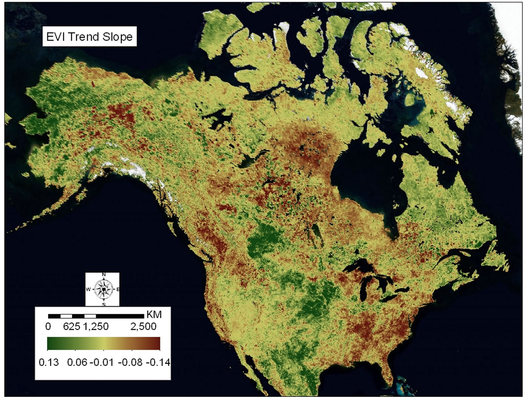

Figure 4. Continental maps of the slope and R2 values for the growing season EVI time-series from 2000- 2010. R2 values ≥ 0.37 carry a 95% confidence level of significance for a two-tailed t-test.

Figure 5. Spatial distribution of trend classes in post-fire forest ecosystems across North America from 2000 through 2010.
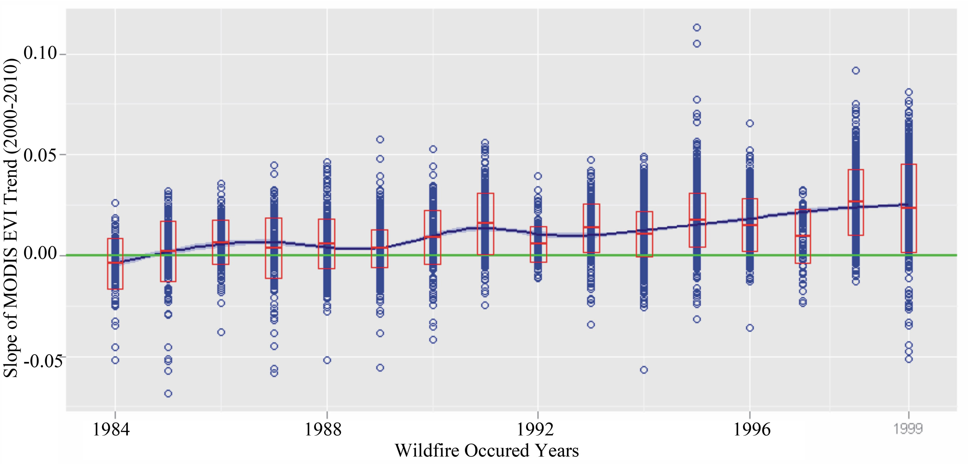
Figure 6. Change in the EVI slope with time since wildfire. The red boxes show the mean and 95% confidence interval of the growing season EVI slope.

Table 2. Post-fire EVI trend dynamics according to post-fire forest age intervals. Positive and negative trends carry a 95% confidence level of significance.
each of these wildfire perimeters showed a negative seasonal EVI trend form 2000 to 2010. These wildfire areas in Table 3 were documented as the most relevant sites for future evaluation studies of the possible causes of delayed or arrested post-fire regrowth of forest vegetation in North America.
4.2. Break Point Detection of Negative EVI Trends
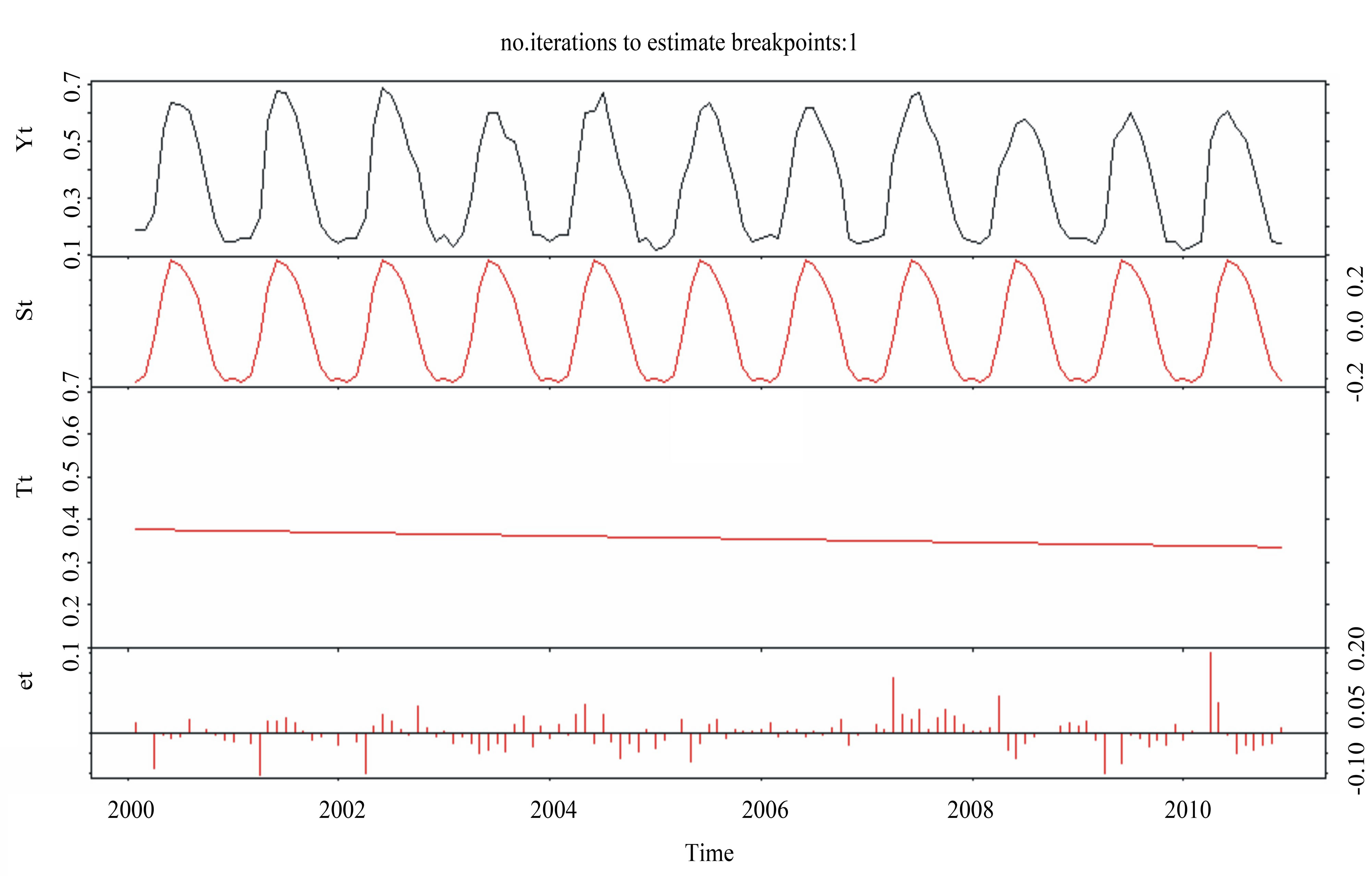
We conducted break point analysis on all 103 pixels in North America with significant negative EVI trends (examples shown in Figure 7). About 15% of all negative trend areas with zero break points implied that the EVI trends of these post-fire areas declined gradually and consistently during the MODIS observation period (2000-2010). The other 85% (Table 4) of all negative trend areas detected with one or more break point over past decade appear to have had vegetation recovery interrupted by some external factor (e.g., extreme weather events), commonly leading to a sudden decline in growing season EVI (e.g., Figure 7(d)).
4.3. Post-Fire Negative EVI and Climate Associations
The linear trends from 2000 to 2010 in three annual climate indices (CMI, SPI and GDD) were examined together, pixel-by-pixel, with growing season MODIS EVI trends. In each set of Figures 8-10, we first plotted the slope of growing season EVI trends against the climate index trends for all post-fire pixel areas, and then for just the significant negative slopes of growing season EVI trends broken-out into the three post-fire age inter vals (Table 2).
A strong association was observed between the trend of annual CMI and post-fire negative EVI trends (Figure 8). More than 78% of significant negative EVI trends were associated with relative drying trends (i.e., negative CMI slope values). The older the post-fire forest, the
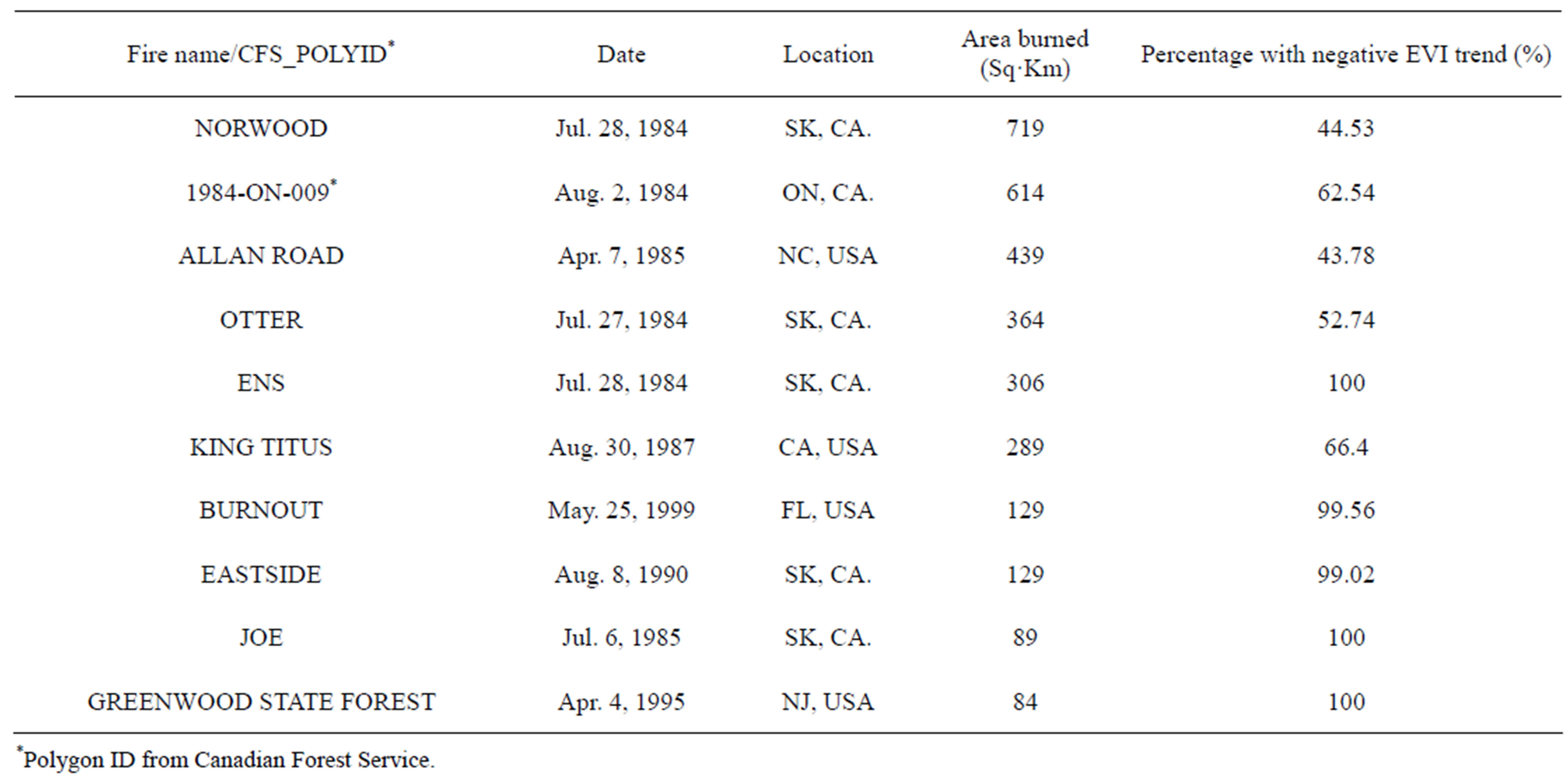
Table 3. Top 10 wildfires in North America (1984-1999) ranked according to the negative EVI trend area within the wildfire perimeter.
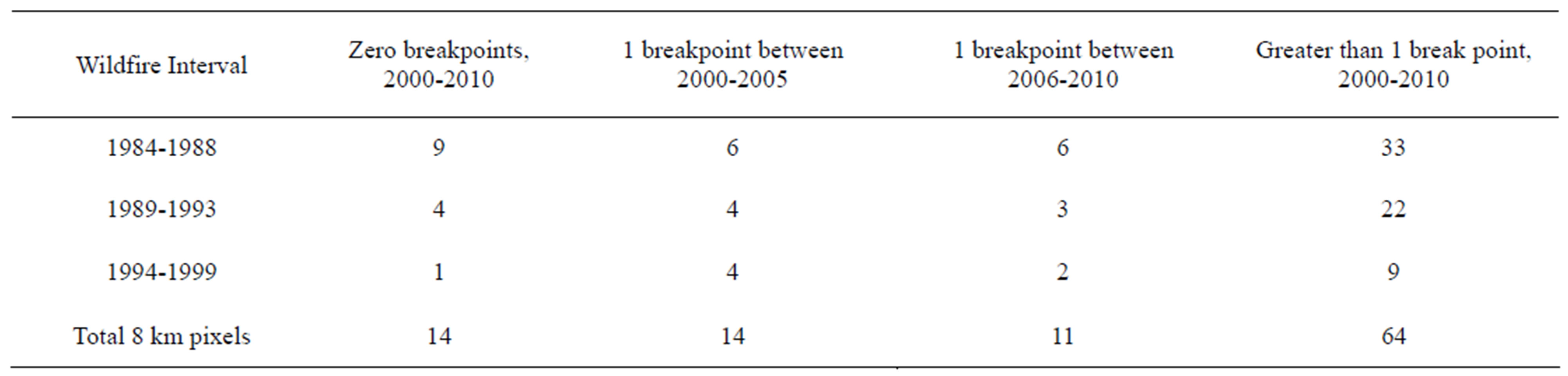
Table 4. Statistics of the BFAST break point results for post-fire pixels with significant negative EVI trends.
 (a)
(a)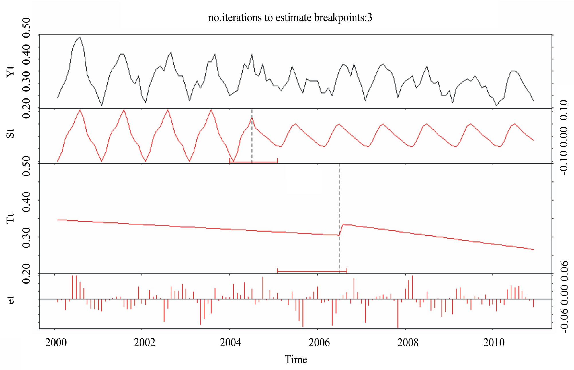 (b)
(b)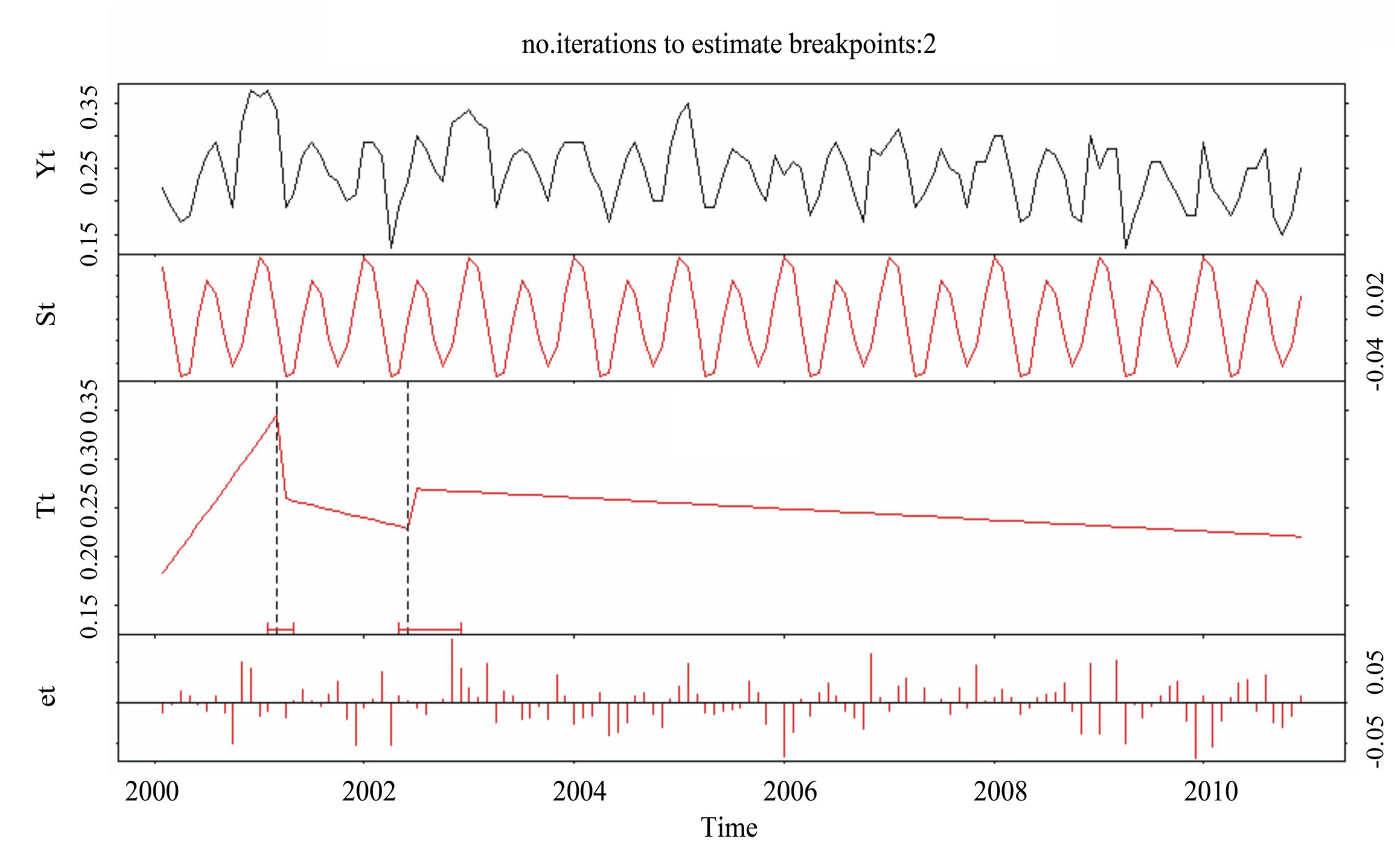 (c)
(c)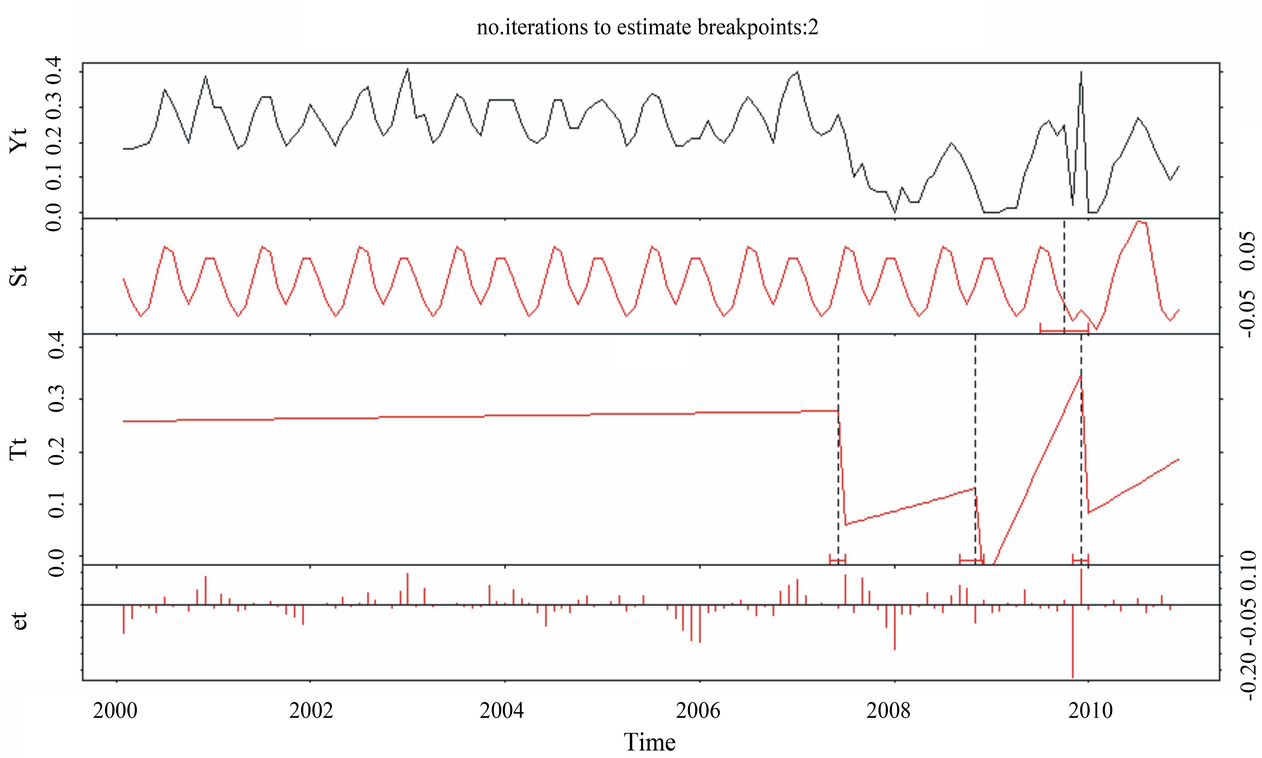 (d)
(d)
Figure 7. Negative EVI trend with break points detected by the BFAST methodology. Examples include: (a) No break points; (b) One break point; (c) Two break points; (d) Three break points. Yt is the time-series MODIS EVI value; St is the fitted seasonal component; Tt is the fitted trend component; et is the noise component.
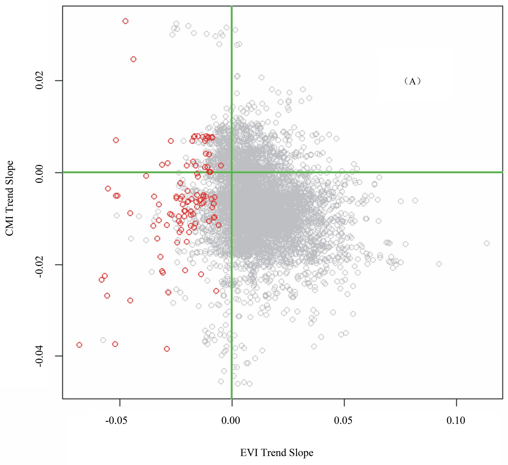
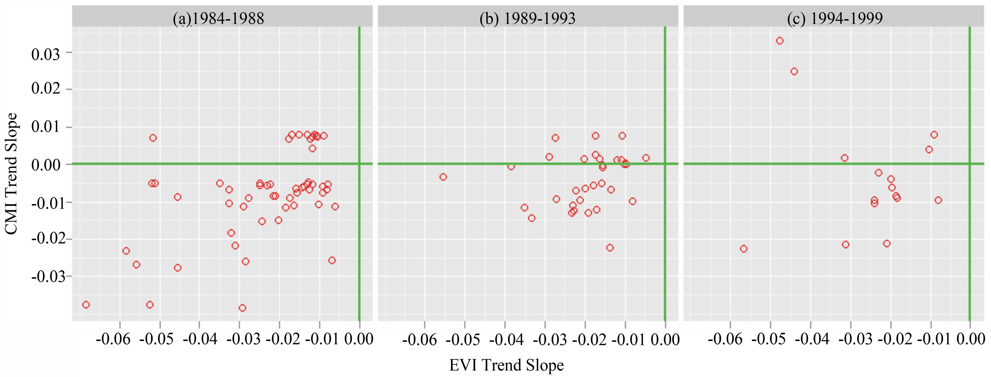
Figure 8. Associations of the trends (2000-2010) in 8 km EVI and annual CMI for all post-fire (1984-1999) pixel areas in North America. Significant negative EVI pixels are shown in red circles, while all other EVI pixels trends are shown in grey circles.
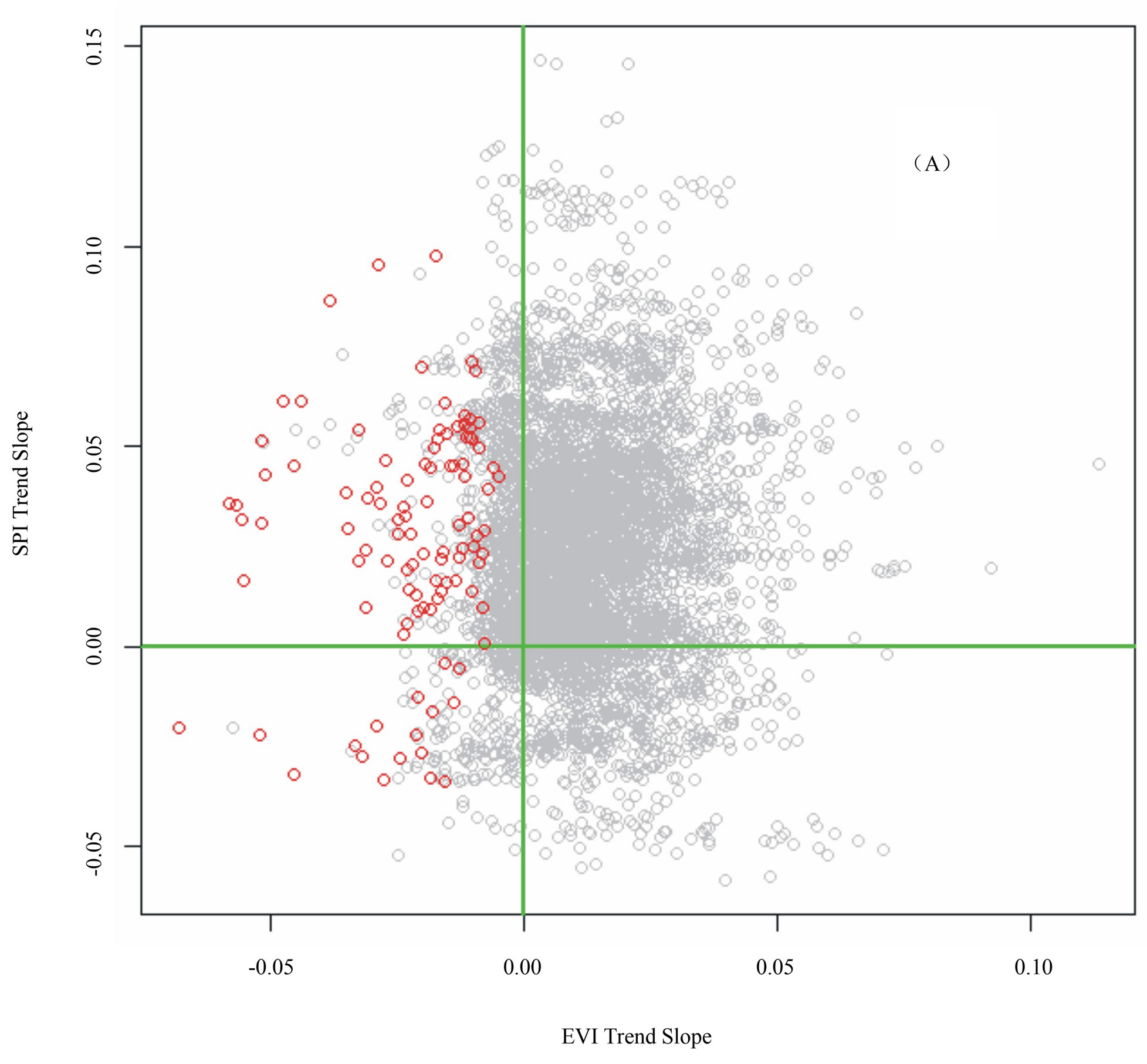
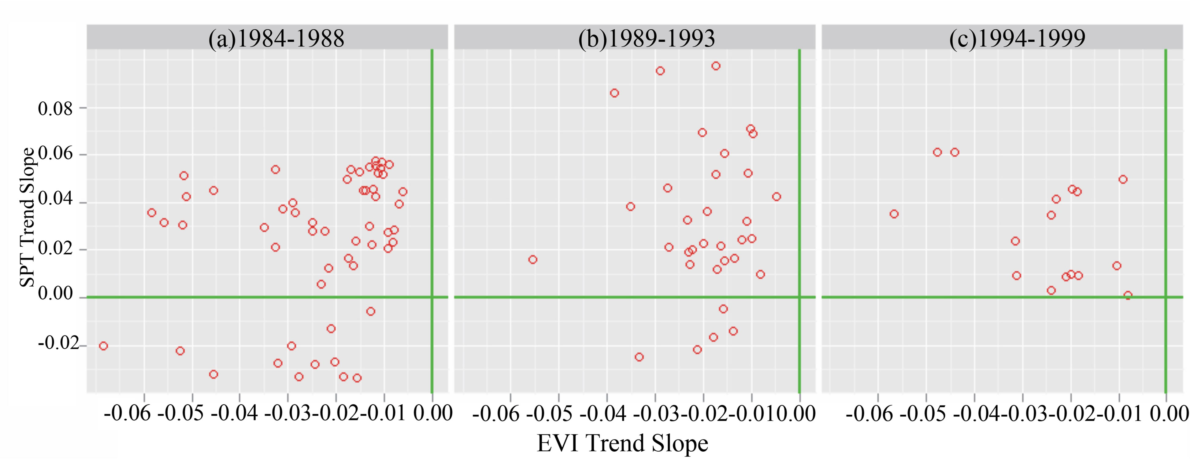
Figure 9. Associations of the trends (2000-2010) in 8 km EVI and annual SPI for all post-fire (1984-1999) pixel areas in North America. Significant negative EVI pixels are shown in red circles, while all other EVI pixels trends are shown in grey circles.

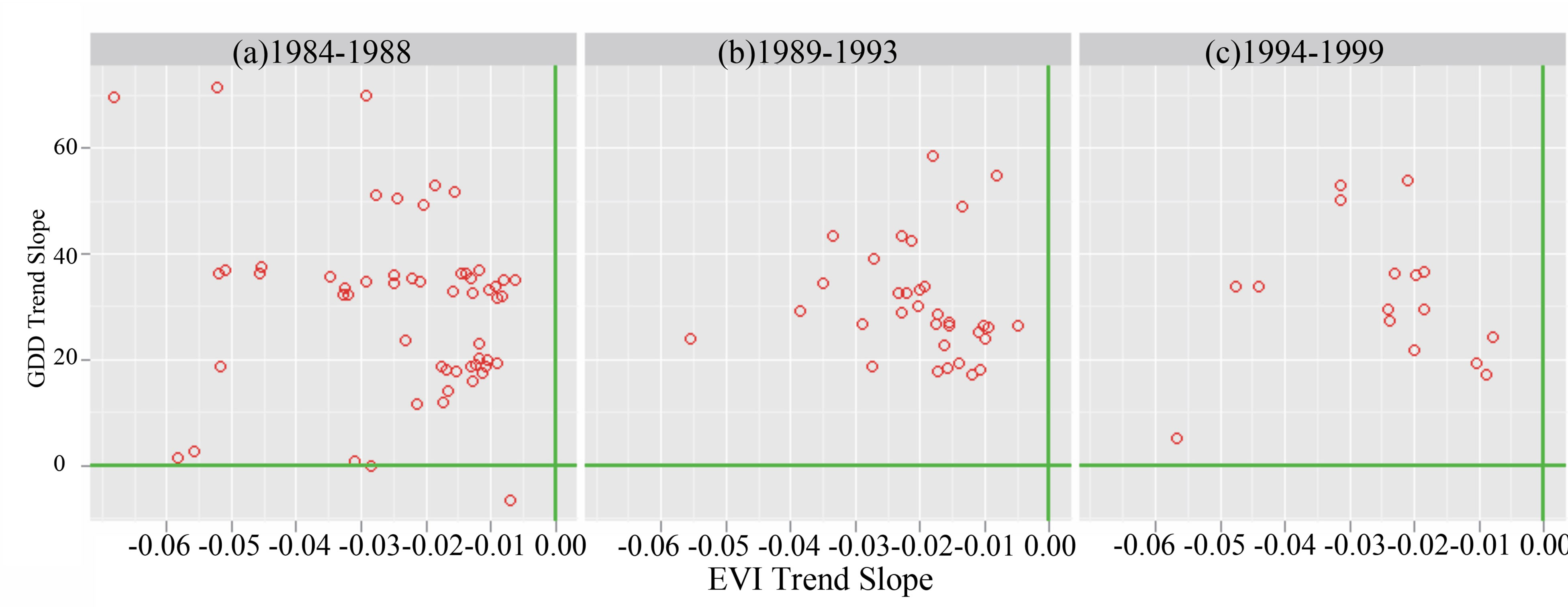
Figure 10. Associations of the trends (2000-2010) in 8-km EVI and annual GDD for all post-fire (1984-1999) pixel areas in North America. Significant negative EVI pixels are shown in red circles, while all other EVI pixels trends are shown in grey circles.
stronger the CMI association with the negative EVI trend. SPI is a ratio of the current precipitation to the historical average precipitation. As was the case with CMI, the older the post-fire forest, the stronger the SPI association with the negative EVI trend (Figure 9).
The more positive the slope value of GDD (base 0˚C), the stronger the warming trend over the past decade (2000-2010) at the post-fire MODIS pixel locations. We found that the overall association between GDD trends and post-fire negative EVI trends was not as strong as the association with CMI trends. However, the more recent wildfire areas (1989-1999) showed less scatter and a more consistent association between GDD trends and post-fire negative EVI trends than the older wildfire areas (1984-1988).
5. DISCUSSION
We have examined a decade of MODIS EVI trends in post-fire forests across North America to determine if vegetation regrowth trends can provide evidence of ongoing climate change impacts. It is generally asserted that anthropogenic climate change will lead to widespread and more frequent forest fires [30]. The increasing wildfire frequency observed across North America in past a few decades can be seen in Figure 2 of our study. An increase in disturbance frequency is likely to increase the rate at which natural vegetation must respond (positively or negatively) to future climate change.
Climate factors may have indirect effects on the recovery of productivity in post-fire forest ecosystems. Insect outbreaks related to warming have been reported by [31,32]. These earlier studies suggested that insect populations were influenced by effects of climate warming and drying on plant community associations and host-tree vigor [32]. Post-fire forest areas are vulnerable and perhaps more sensitive than mature natural forests to insect damage, although little evidence is available to quantify this explanation. Nonetheless, the results of CMI trend associations from our study are consistent with insect damage effects on EVI patterns.
The Normalized Difference Vegetation Index (NDVI) derived from AVHRR time-series data has been used by previous studies for post-fire trends [2,8,14,]. Compared to the traditional AVHRR NDVI time-series product, there are advantages in using monthly MODIS EVI time-series dataset for the retrieval of post-fire forest trends. EVI has the ability to better eliminate canopy background and atmosphere noise, which are typical NDVI limitations [16]. EVI is an optimized index designed to enhance the vegetation signal with improved vegetation monitoring ability. The EVI is more responsive to canopy structural variations, including leaf area index (LAI), canopy type, plant physiognomy, and canopy architecture, while NDVI is mainly chlorophyllsensitive. The main limitation of using EVI time-series data is that MODIS data acquired only spans the latest decade. The first results from our study of the years 2000 to 2010 can provide a baseline for long-term (>10 years) climate change and forest regrowth studies in years to come.
6. CONCLUSION
The MODIS EVI time-series data used in this study provided consistent large-scale metrics of post-fire forest regrowth trends across North America. Temperature warming-induced change and variability of precipitation at local and regional scales may have altered the trends of large post-fire forest regrowth and could be impacting the resilience of post-fire forest ecosystems in North America. The methodology developed for mapping and characterization of forest regrowth trends can be readily extended over the next decade of MODIS EVI data. The results from BFAST break point analysis provides an effective trend decomposition method for local scale studies with higher resolution satellite data. Further research should be pursued in order to elucidate the developing relationship between post-fire forest regrowth and ongoing climate change.
7. ACKNOWLEDGEMENTS
This work was conducted with the support from NASA under the U. S. National Climate Assessment. This research was also supported by an appointment of the first author to the NASA Postdoctoral Program at the NASA Ames Research Center, administered by Oak Ridge Associated Universities. We thank Cyrus Hiatt, Vanessa Genovese, and Steven Klooster of California State University Monterey Bay for assistance with regional data sets and programming.
REFERENCES
- Amiro, B.D., Chen, J.M. and Liu, J. (2000) Net primary productivity following forest fire for Canadian ecoregions. Canadian Journal of Forest Research, 30, 939-947. doi:10.1139/x00-025
- Casady, G.M. and Marsh, S.E. (2010) Broad-scale environmental conditions responsible for post-fire vegetation dynamics. Remote Sensing, 2, 2643-2664. doi:10.3390/rs2122643
- Cuevas-GonzALez, M., Gerard, F., Balzter, H. and RiaNO, D. (2009) Analysing forest recovery after wildfire disturbance in boreal Siberia using remotely sensed vegetation indices. Global Change Biology, 15, 561-577. doi:10.1111/j.1365-2486.2008.01784.x
- Epting, J. and Verbyla, D.L. (2005) Landscape level interactions of pre-fire vegetation, burn severity, and post-fire vegetation over a 16-year period in interior Alaska. Canadian Journal of Forest Research, 35, 1367- 1377. doi:10.1139/x05-060
- Pickett, S.T.A. and White, P.S. (1985) The ecology of natural disturbances and patch dynamics. Academic Press, Orlando.
- Overpeck, J.T., Rind, D. and Goldberg, R. (1990) Climate-induced changes in forest disturbance and vegetation. Nature, 343, 51-53. doi:10.1038/343051a0
- Westerling, A.L., Hidalgo, H.G., Cayan, D.R. and Swetnam, T.W. (2006) Warming and earlier spring increase western US forest wildfire activity. Science, 313, 940-943. doi:10.1126/science.1128834
- Goetz, S.J., Fiske, G.J. and Bunn, A.G. (2006) Using satellite time-series data sets to analyze fire disturbance and forest recovery across Canada. Remote Sensing of Environment, 101, 352-365. doi:10.1016/j.rse.2006.01.011
- Baldocchi, D., Falge, E., Gu, L.H., Olson, R., Hollinger, D., Running, S., et al. (2001) FLUXNET: A new tool to study the temporal and spatial variability of ecosystem-scale carbon dioxide, water vapor, and energy flux densities. Bulletin of the American Meteorological Society, 82, 2415-2434. doi:10.1175/1520-0477(2001)082<2415:FANTTS>2.3.CO;2
- McGuire, A.D., Sitch, S. and Wittenberg, U. (2001) Carbon balance of the terrestrial biosphere in the twentieth century: Analyses of CO2, climate, and land use effects with four process-based ecosystem models. Global Biogeochemical Cycles, 15, 183. doi:10.1029/2000GB001298
- Kasischke, E.S. and French, N.H.F. (1997) Constraints on using AVHRR composite index imagery to study patterns of vegetation cover in boreal forests. International Journal of Remote Sensing, 18, 2403-2426. doi:10.1080/014311697217684
- Amiro, B.D., MacPherson, I.J., Desjardins, R.L., Chen, J.M. and Liu, J. (2003) Post-fire carbon dioxide fluxes in the western Canadian boreal forest: Evidence from towers, aircraft and remote sensing. Agricultural and Forest Meteorology, 115, 91-107. doi:10.1016/S0168-1923(02)00170-3
- Brown, M.E., Pinzon, J.E. and Tucker, C.J. (2004) New vegetation index data set to monitor global change. American Geophysical Union EOS Transactions, 85, 565- 569. doi:10.1029/2004EO520003
- Goetz, S.J., Bunn, A.G., Fiske, G.J. and Houghton, R.A. (2005) Satellite observed photosynthetic trends across boreal North America associated with climate and fire disturbance. Proceedings of the National Academy of Sciences, 103, 13521-13525. doi:10.1073/pnas.0506179102
- LP-DACC: NASA Land Processes Distributed Active Archive Center (2007) MODIS/Terra vegetation indices monthly L3 global 0.05Deg CMG (MOD13C2), Version 005, USGS/Earth Resources Observation and Science (EROS) Center, Sioux Falls.
- Huete, A., Didan, K., Miura, T., Rodriquez, E., Gao, X. and Ferreira, L. (2002) Overview of the radiometric and biophysical performance of the MODIS vegetation indices. Remote Sensing of Environment, 83, 195-213. doi:10.1016/S0034-4257(02)00096-2
- Eidenshenk, J., Schwind, B., Brewer, K., Zhu, Z., Quayle, B. and Howard, S. (2007) A project for monitoring trends in burn severity. Fire Ecology, 3, 3-21.
- Canadian Forest Service (2010) National fire database— Agency fire data. Natural Resources Canada, Canadian Forest Service, Northern Forestry Centre, Edmonton.
- Homer, C., Dewitz, J., Fry, J., Coan, M., Hossain, N., Larson, C., Herold, N., McKerrow, A., VanDriel, J.N. and Wickham, J. (2007) Completion of the 2001 national land cover database for the conterminous United States. Photogrammetric Engineering and Remote Sensing, 73, 337- 341.
- Kalnay, E., Kanamitsu, M., Kistler, R., Collins, W., Deaven, D., Gandin, L., Iredell, M., Saha, S., White, G., Woollen, J., Zhu, Y., Leetmaa, A., Reynolds, B., Chelliah, M., Ebisuzaki, W., Higgins, W., Janowiak, J., Mo, K.C., Ropelewski, C., Wang, J., Jenne, R. and Joseph, D. (1996) The NCEP/NCAR 40-year reanalysis project. Bulletin of the American Meteorological Society, 77, 437-472. doi:10.1175/1520-0477(1996)077<0437:TNYRP>2.0.CO;2
- Potter, C., Klooster, S., Hiatt, C., Genovese, V. and Castilla-Rubio J.C. (2011) Changes in the carbon cycle of Amazon ecosystems during the 2010 drought. Environmental Research Letters, 6, 034024. doi:10.1088/1748-9326/6/3/034024
- Potter, C.S. and Brooks, V. (1998) Global analysis of empirical relations between annual climate and seasonality of NDVI. International Journal of Remote Sensing, 19, 2921-2948. doi:10.1080/014311698214352
- Willmott, C.J. and Feddema, J.J. (1992) A more rational climatic moisture index. Professional Geographer, 44, 84-88. doi:10.1111/j.0033-0124.1992.00084.x
- McKee, T.B., Doeskin, N.J. and Kieist, J. (1993) The relationship of drought frequency and duration to time scales. Proceedings of 8th Conference on Applied Climatology, Boston, 17-22 January 1993, 179-184.
- Guttman, N.B. (1999) Accepting the standardized precipitation index: A calculation algorithm. Journal of the American Water Resources Association, 35, 311-322. doi:10.1111/j.1752-1688.1999.tb03592.x
- Verbesselt, J., Hyndman, R., Newnham, G. and Culvenor, D. (2010) Detecting trend and seasonal changes in satellite image time series. Remote Sensing of Environment, 114, 106-115. doi:10.1016/j.rse.2009.08.014
- Verbesselt, J., Hyndman, R., Zeileis, A. and Culvenor, D. (2010) Phenological change detection while accounting for abrupt and gradual trends in satellite image time series. Remote Sensing of Environment, 114, 2970-2980. doi:10.1016/j.rse.2010.08.003
- Crist, E.P. and Cicone, R.C. (1984). A physically-based transformation of thematic mapper data—The TM tasseled cap. IEEE Transactions on Geoscience and Remote Sensing, 22, 256-263. doi:10.1109/TGRS.1984.350619
- Anyamba, A. and Eastman, J.R. (1996). Interannual variability of NDVI over Africa and its relation to El Nino southern oscillation. International Journal of Remote Sensing, 17, 2533-2548. doi:10.1080/01431169608949091
- Parry, M.L., Canziani, O.F., Palutikof, J.P., van der Linden, P.J. and Hanson, C.E., Eds. (2007) Climate change 2007: Impacts, adaptation and vulnerability. Cambridge University Press, Cambridge.
- Aukema, B.H., Carroll, A.L., Zheng, Y., Zhu, J., Raffa, K.F., Moore, R.D., Stahl, K. and Taylor, S.W. (2008) Movement of outbreak populations of mountain pine beetle: Influence of spatiotemporal patterns and climate. Ecography, 31, 348-358. doi:10.1111/j.0906-7590.2007.05453.x
- Bentz, B.J., Regniere, J., Fettig, C.J., Hansen, E.M., Hayes, J.L., Hicke, J.A., et al. (2010) Climate change and bark beetles of the western United States and Canada: Direct and indirect effects. BioScience, 60, 602-613. doi:10.1525/bio.2010.60.8.6