Natural Science
Vol.4 No.7(2012), Article ID:20767,4 pages DOI:10.4236/ns.2012.47057
Species and global change—Assessing the extinction point of albacore stocks
![]()
1Biological and Fishery Division, Institute of Oceanography, National Taiwan University, Taipei, Chinese Taipei; *Corresponding Author: chwang@ntu.edu.tw
2Institute of Marine Resource Management, College of Life and Resource, Sciences, National Taiwan Ocean University, Keelung, Chinese Taipei; sbwang@mail.ntou.edu.tw
Received 11 May 2012; revised 10 June 2012; accepted 24 June 2012
Keywords: Global change; environment; carrying capacity; extinction; albacore; biomass; estimation of carrying capacity
ABSTRACT
Global change determines the environmental condition and leads to decide the carrying capacity. While carrying capacity determines the extinction of the species, it is an important issue to estimate the extinction point of the species, the minimal carrying capacity, or the tolerant limitation of the species. If it is possible to estimate the tolerant limitation of the species, it will be possible to control the global change. Applied the above idea to the albacore stocks, it revealed that extinction point was about 0.0018% of the present status. From these results, it implies that this method may also suitable to other species for estimating their carrying capacities.
1. INTRODUCTION
In the 21-st century, global change is the most serious problem for human life. Besides of the lack of food, floods, drought, typhoon, mudflows, or landslides, and so on, certainly, the damage of global change is remarkable. Different species naturally have different responses for varied environments. They need to suit in and get adapted to different environments. Varied environments determine the carrying capacity of the species and induce the fluctuation of the population. Carrying capacity provides the necessary information about the response of the species under global change. Stable environment implies stable carrying capacity while worse environment shows smaller carrying capacity and better environment gets larger carrying capacity.
In fishery, definition of the carrying capacity was “the maximum equilibrium population biomass to which the population will approach in the absence of interference” (Gulland [1]). It was always with extensive, but imprecise, and different meanings in many research fields. The variability was due to it entailed a myriad of interrelating, ever changing biotic and non-biotic factors (Monte-Luna [2], Mora [3], Tittensor [4], Mora [5], Mora [6]). However, it is a well-defined index of the species responding to the environmental condition.
Schaefer model (Schaefer [7], Schaefer [8]) provided a useful tool for estimating the carrying capacity. It always showed a symmetric relationship between net production and biomass. Pella and Tomlinson (Pella and Tomlinson, [9]) suggested a generalized production model by adding a curve parameter in Schaefer model. Although, it applied extensively in non-symmetric curve, curve parameter was not necessary and non-symmetric curve was depending on varied carrying capacity (Wang and Wang [10]).
Any species need to adapt themselves continuously to variable environment. The South Pacific albacore stock was deeply depending on the sea surface temperature (Wang [11], Wang [12]). Wang (Wang [13]) showed that consuming the available food sufficiently was the best life strategies. Global change determines the environment and the same to the carrying capacity. This paper tried to estimate the extinction point of the species based on carrying capacity.
2. ESTIMATION OF CARRYING CAPACITY
If reliable catch and effort are available and fishing efforts could standardize sufficiently, Schaefer model was a useful tool for estimating the carrying capacity (Wang and Wang [10]). The method summarized as follows.
Schaefer (Schaefer [7], Schaefer [8]) provided a useful model for assessing fish stocks.
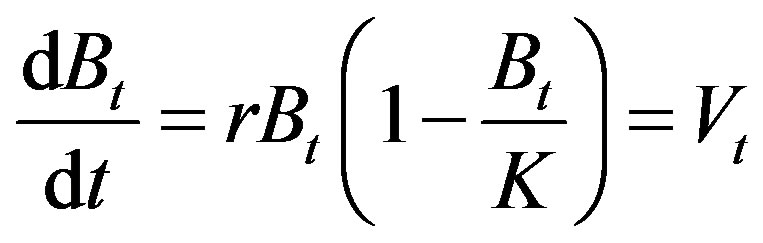 (1)
(1)
where Vt = net production at time t, Bt = biomass at time t, r = intrinsic growth rate, K = carrying capacity. Positive, negative or zero of Vt means increasing, decreasing or stable of the biomass, respectively.
Under fishing, eq.1 becomes
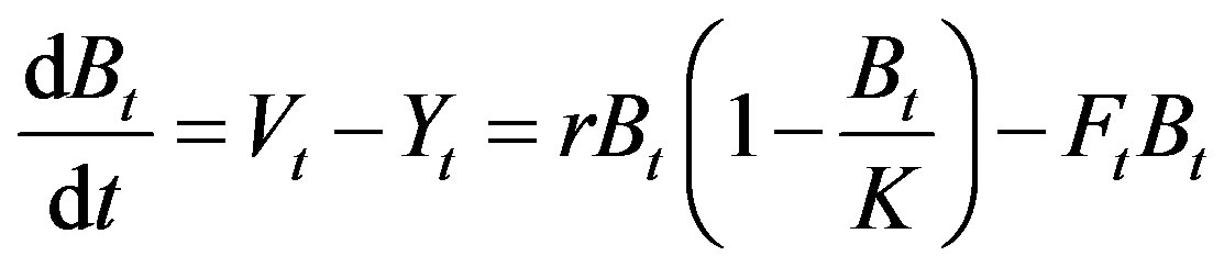 (2)
(2)
where Ft = fishing mortality rate at time t, Yt = catch at time t. Setting F to be constant in one year and integrating eq.2, the annual catch is available as follows:
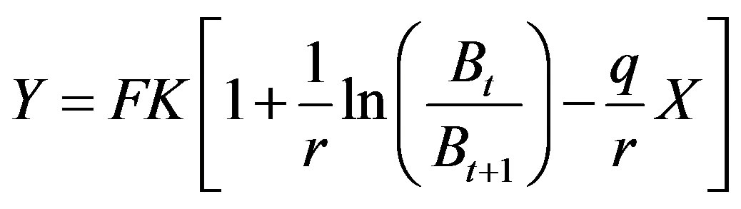 (3)
(3)
where F = qX with q = catch ability, X = fishing effort, Bt = biomass at the beginning of this year, Bt+1 = biomass at the end of this year. Under equilibrium catch,  implies
 (4)
(4)
where U = = catch per unit of fishing effort.
Generally, q is set to be constant after standardized fishing efforts sufficiently. Intrinsic growth rate r means the inherent ability of the reproduction and growth of this species. Generally, it sets to be constant. Carrying capacity depends on environment and varies year by year. Therefore, eq.3 should rewrite as follows.
or
 (5)
(5)
where  catch per unit of fishing effort. For stable eivironment, naturally carrying capacity is constant, say
  for all i-year. It implies eq.6.
 (6)
(6)
This equation can use to estimate parameters r, q, and Kc as follows:
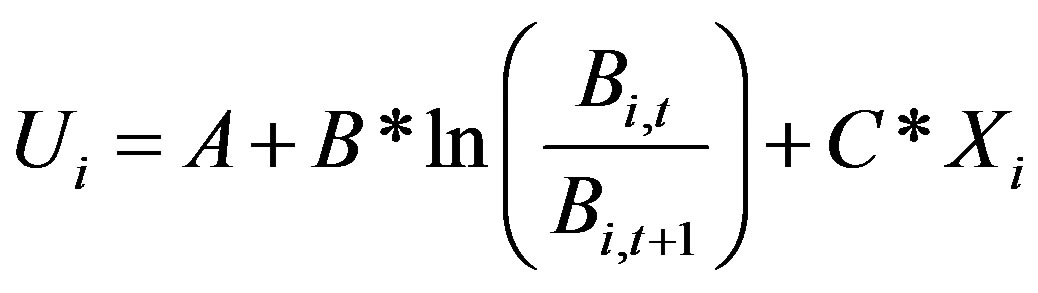 (7)
(7)
where
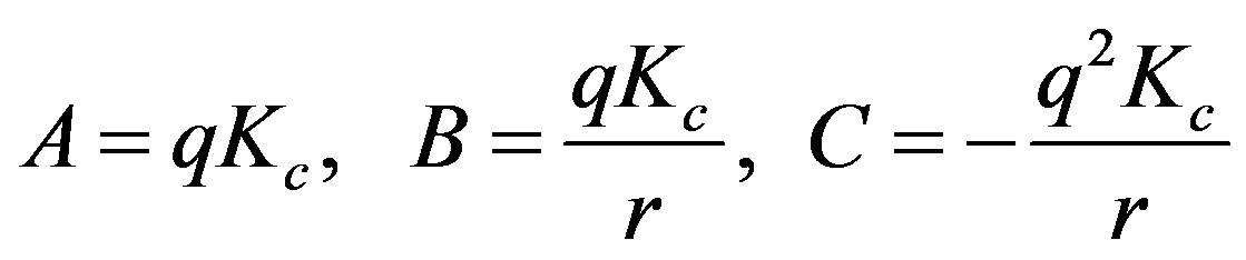
Set  and
and 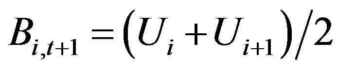 then A, B, and C are available by the method of least squares as
 .
.
3. RESPONDING TO THE ENVIRONMENT
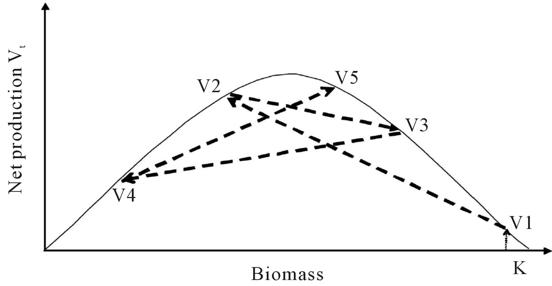
Theoretically, Schaefer model (Schaefer [7], Schaefer [8]) provided a symmetric curve of the relationships between net production and biomass. Applying to assessing fish stock, the symmetric curve was generally unavailable. Pella and Tomlinson (Pella and Tomlinson [9]) suggested a curve parameter for fitting the non-symmetric curve. However, non-symmetric curve was also available with variable carrying capacities (Figure 1). In population dynamics, the species need to adjust the fecundity, survival rate and/or growth rate responding to varied environments. As shown in Figure 2, any change of the fecundity, survival rate and/or growth rate will skew the curve. It indicated that the curve parameter is not necessary. However, variable m determined the skew curve and responding to the varied carrying capacity. It indicates that m should be necessary and meaningful biological index. It seems reasonable to rewrite equation (1) by adding a new index m as follows.
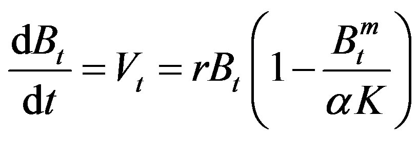 (8)
(8)
As shown above, m is an index reflecting the variables environments. For the present status, naturally it is m = 1 and α = 1. Better environment (α > 1) implies m > 1. Contrary, worse environment (α < 1) implies m < 1. Under extremely bad environment with α approaching zero then m will evenly become negative. Negative m means that the environment is so bad even over the tolerant limit of the species. Clearly, m > 1 is comparatively inactive depending on the varied environments. However, it is sharply reflecting to the environments as m < 1 as shown in Figure 3. It seems indicating that m is an adaptation index reflecting to the varied environments. The adaptation rate m is a short-term index corresponding to the intrinsic growth rate r the long-tern index of the species.
Naturally, all species will close to extinction if the environment is extremely bad. This is available when m = 0 with net production always be negative. This is the absolute extinction point of the species. On the other hand, Eq.1 reveals that negative net production is available while the environment becomes so bad with carrying capacity lower than the biomass. If it is continuously then the species is also approaching extinction. It implies that  is the relative extinction point.
For south Pacific albacore stocks, the present status is
 (a)
(a)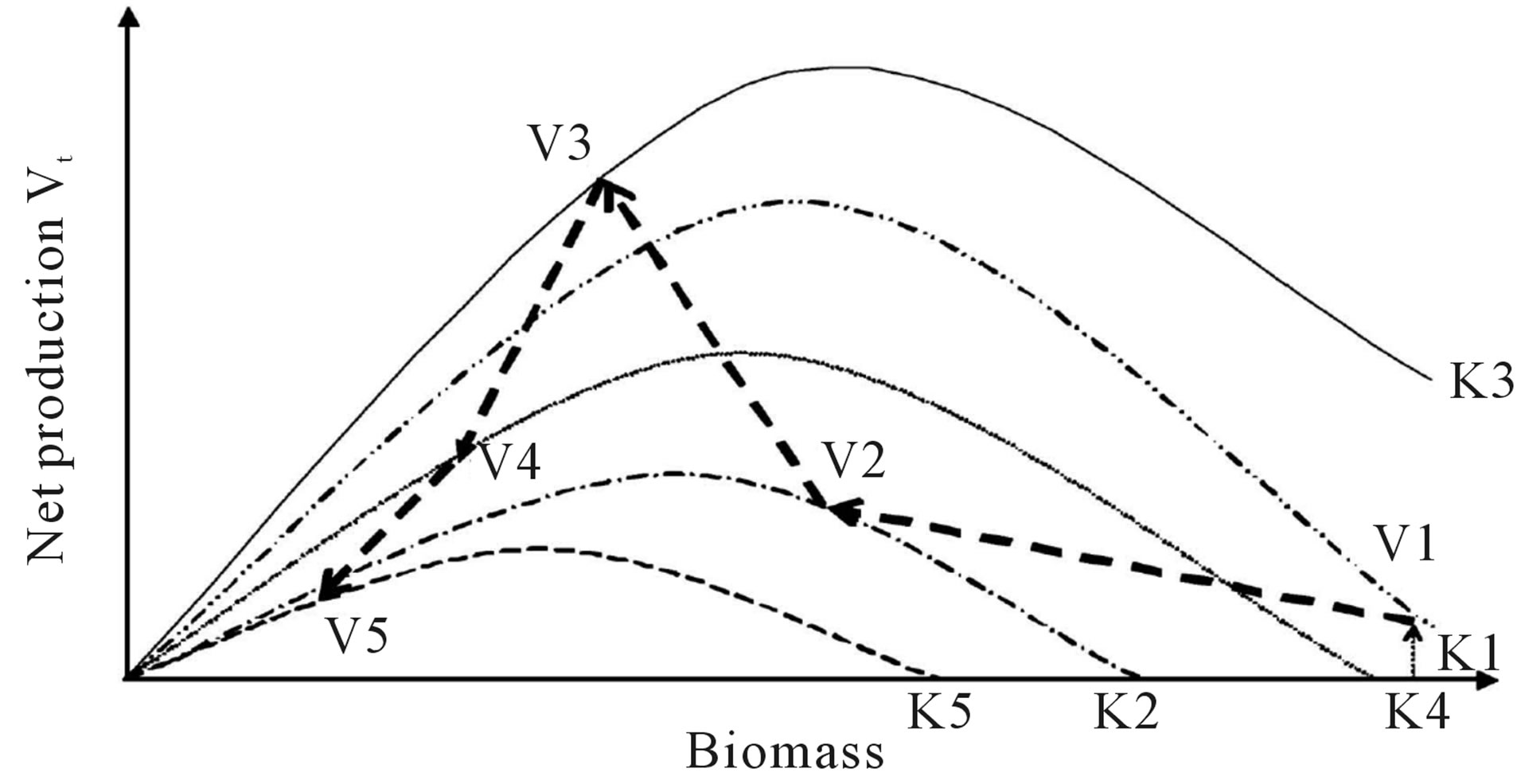 (b)
(b)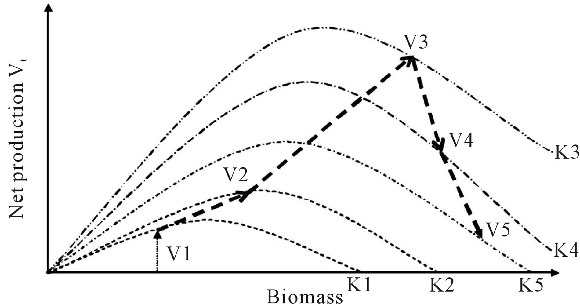 (c)
(c)
Figure 1. (a) Symmetric parabola curve if stable carrying capacity K with net production varied as: V1 V2
V2 V3
V3 V4
V4  V5; (b) Mod skewed to the left when carrying capacity changed as: K1
 K2
K2 K3
K3 K4
K4 K5 and net production varied as: V1
 V2
V2 V3
V3 V4
V4 V5; (c) Mod skewed to the right when carrying capacity changed as: K1
 K2
K2 K3
K3 K4
K4 K5 and net production varied as: V1
 V2
V2 V3
V3 V4
V4  V5.
V5.
about r = 1.28374, K = 97,985 metric tons, V = 30,789 metric tons and B = 56,079 metric tons (Wang and Wang [10]). For the present status, net production will become negative as α = 0.572. This is the relative extinction point of albacore stocks. If the environment is extremely bad with α = 0.000017 only, then m near to zero. This is the absolute extinction point of the albacore stocks.
4. DISCUSSIONS AND CONCLUSIONS
All species need to adapt themselves to the variable
 (a)
(a)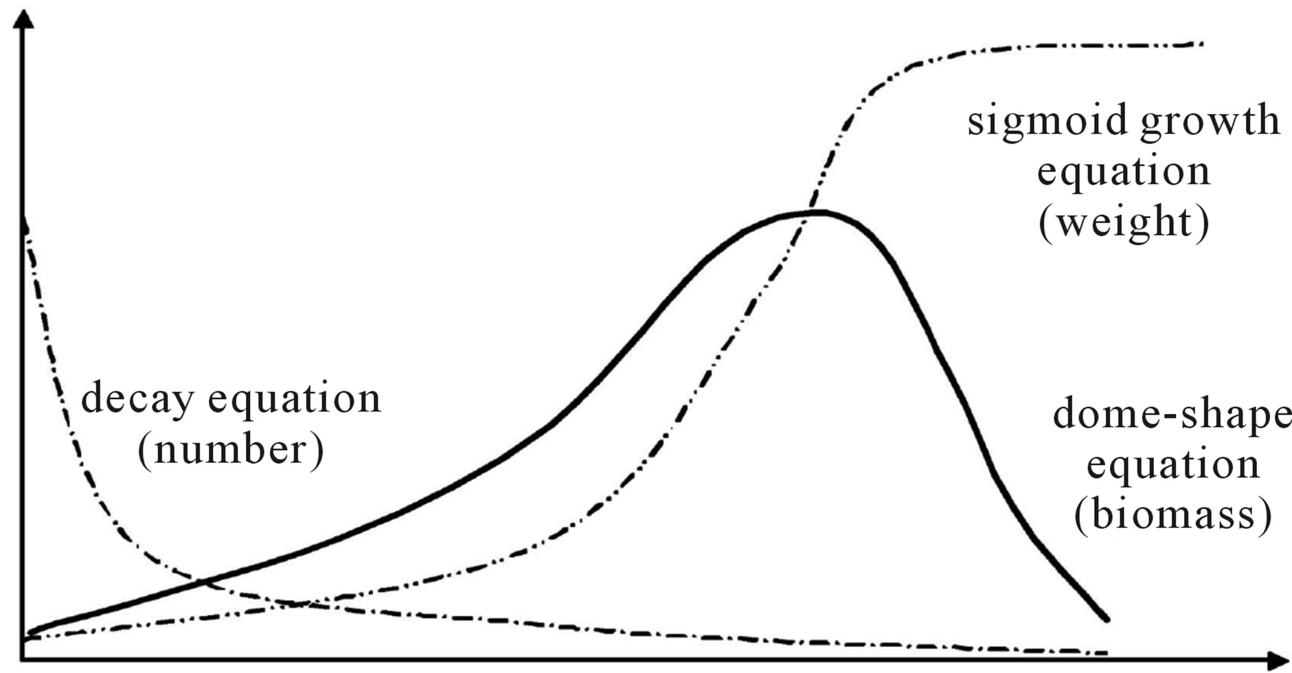 (b)
(b)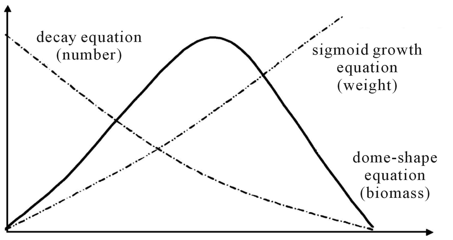 (c)
(c)
Figure 2. (a) Mod skewed to the left due to better environments; (b) Mod skewed to the right due to better environments; (c) Symmetric parabola curve under comparatively stable environments.
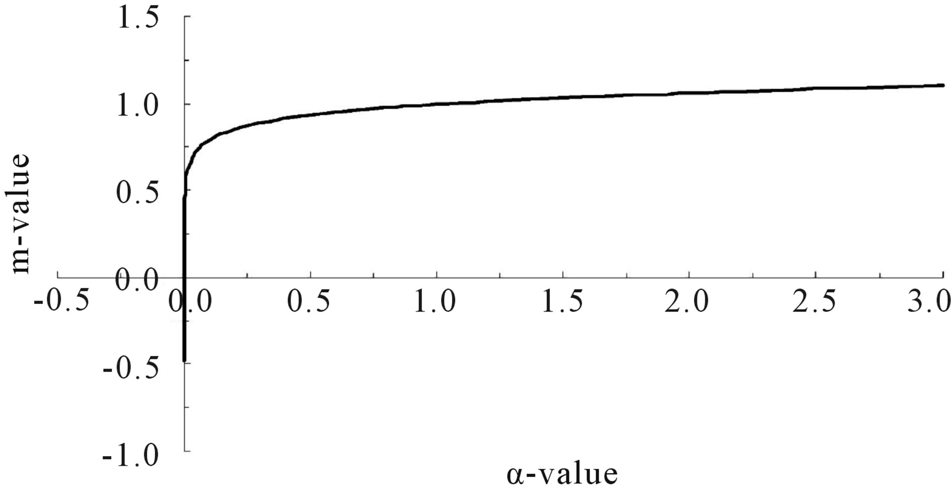
Figure 3. Adaptation index corresponding to the varied carrying capacity.
environments or they will disappear gradually from the earth. Violent environment is naturally unappreciable. However, stable environment is always unavailable. Any decreasing of the carrying capacity implies the worse environment while increasing of the carrying capacity indicates the better environments. Relative extinction point provides the important information of the present status of the species. On the other hand, the absolute extinction point provides the important information of the tolerant limit of that species.
Global change is so important in the coming century. Due to different species appreciated different environments, it is not so easy to assess whether the global change is merit or damage. It seems necessary to choose some indicator species for assessing the influence of the global change. This study come out a predictable method for species faced and adjusted to the global change.
REFERENCES
- Gulland, J.A. (1983) Fish stock assessment, a manual of basic models. John Wiley & Sons, Chichester, New York, Brisbane, Toronto, Singapore.
- Del Monte-Luna, P., Brook, B.W., Zetina-Rejon, M. and Cruz-Escalona, V.H. (2004) The carrying capacity of ecosystem. Global Ecological Biogeography, 13, 485-495. doi:10.1111/j.1466-822X.2004.00131.x
- Mora, C. and Sale, P. (2011) Ongoing global biodiversity loss and the need to move beyond protected areas: A review of the technical and practical shortcoming of protected areas on land and sea. Marine Ecology Progress Series, 434, 251-266. doi:10.3354/meps09214
- Tittensor, D., Mora, C., Jetz, W., Lotze, H.K., Ricard, D., vanden Berghe, E. and Worm, B. (2010) Global patterns and predictors of marine biodiversity across taxa. Nature, 466, 1098-1101. doi:10.1038/nature09329
- Mora, C., Myers, R., Pitcher, T., Zeller, D., Watson, G., Sumila, R., Gaston, K. and Worm, B. (2009) Management effectiveness of the world’s marine fisheries. PLoS Biology, 7, e1000131. doi:10.1371/journal.pbio.1000131
- Mora, C., Metzker, R., Rollo, A. and Myers, R.A. (2007) Experimental simulations about the effects of habitat fragmentation and overexploitation on populations facing environmental warming. Proceedings of the Royal Society of London B, 274, 1023-1028. doi:10.1098/rspb.2006.0338
- Schaefer, M.B. (1954) Some aspects of the dynamics of populations, important for the management of the commercial marine fisheries. Inter-American Tropical Tuna Commission, 1, 7-56.
- Schaefer, M.B. (1957) A study of the dynamics of the fishery for yellowfin tuna in the eastern tropical Pacific Ocean. Inter-American Tropical Tuna Commission, 2, 247- 285.
- Pella, J.J. and Tomlinson, P.K. (1969) A generalized stock production model. Inter-American Tropical Tuna Commission, 13, 419-496.
- Wang, C.H. and Wang, S.B. (2006) Assessment of South Pacific albacore stock (Thunnus alalunga) by improved Schaefer model. Journal of Ocean University of China, 5, 147-154.
- Wang, C.H. (1988) Seasonal changes of the distribution of south Pacific albacore based on Taiwan’s tuna longline fisheries, 1971-1985. ACTA Oceanographica Taiwanica, 20, 13-40.
- Wang, C.H. (1999) Fluctuation of the south Pacific albacore stocks (Thynnus alalunga) relative to the sea surface temperature. Terrestrial, Atmospheric and Oceanic Sciences, 10, 341-364.
- Wang, C.H. (1976) Relationship between larval food consumptions and recruitments in fish population. ACTA Oceanographica Taiwanica, 6, 179-188 (in Chinese).