Engineering
Vol.6 No.3(2014), Article ID:43530,14 pages DOI:10.4236/eng.2014.63015
Computational Simulations of Bone Remodeling under Natural Mechanical Loading or Muscle Malfunction Using Evolutionary Structural Optimization Method
Hadi Latifi1, Yi Min Xie1, Xiaodong Huang1, Mehmet Bilgen2
1Centre for Innovative Structures and Materials, School of Civil, Environmental and Chemical Engineering, RMIT University, Melbourne, Australia
2Biophysics Department, Faculty of Medicine, Erciyes University, Kayseri, Turkey
Email: Mehmet.Bilgen@yahoo.com
Copyright © 2014 by authors and Scientific Research Publishing Inc.
This work is licensed under the Creative Commons Attribution International License (CC BY).
http://creativecommons.org/licenses/by/4.0/


Received 25 December 2013; revised 24 January 2014; accepted 3 February 2014
ABSTRACT
Live bone inherently responds to applied mechanical stimulus by altering its internal tissue composition and ultimately biomechanical properties, structure and function. The final formation may structurally appear inferior by design but complete by function. To understand the loading response, this paper numerically investigated structural remodeling of mature sheep femur using evolutionary structural optimization method (ESO). Femur images from Computed Tomography scanner were used to determine the elastic modulus variation and subsequently construct finite element model of the femur with stiffest elasticity measured. Major muscle forces on dominant phases of healthy sheep gait were imposed on the femur under static mode. ESO was applied to progressively alter the remodeling of numerically simulated femur from its initial to final design by iteratively removing elements with low strain energy density (SED). The computations were repeated with two different mesh sizes to test the convergence. The elements within the medullary canal had low SEDs and therefore were removed during the optimization. The SEDs in the remaining elements varied with angle around the circumference of the shaft. Those elements with low SED were inefficient in supporting the load and thus fundamentally explained how bone remodels itself with less stiff inferior tissue to meet load demand. This was in line with the Wolff’s law of transformation of bone. Tissue growth and remodeling process was found to shape the sheep femur to a mechanically optimized structure and this was initiated by SED in macro-scale according to traditional principle of Wolff’s law.
Keywords:Bone Remodeling; Computer Simulation; Finite Element Modeling; Evolutionary Structural Optimization; Wolff’s Law

1. Introduction
Bone has been considered as a “naturally optimum structure” [1] , meaning that healthy bone, according to Wolff’s law, adapts to its conditional mechanical loading or functional stimulus. To uncover this phenomenon, various studies have been conducted to understand the fundamental principles of bone formation and remodeling with age and external factors [1] [2] . The capacity of bone in humans or animals to adapt has been validated to a degree by using scientific tools involving finite element (FE) analysis [3] -[5] . Evolutionary structural optimization (ESO) was originated from structural engineering for achieving best performance from a design under predefined constraints on its material constituents and mechanical expectations [6] . The method is based on the concept of iteratively removing mechanically inefficient material from the underlying structure so that it evolves towards a final design with minimal use of material, while still satisfying the load requirements. A research question that rises is—can ESO be used to understand the adaptation mechanism of a self-developed solid biological material like bone? To address this question, we developed a numerical platform combining ESO with FE analysis. Using this platform, we evaluated macroscopic behavior of sheep femur under loads imposed by a normal walking. Specifically, we implemented Hard-Kill ESO which removes elements with lowest strain energy density (SED). With iterative process, the model was let to evolve toward its final form. This paper describes the preliminary developmental work with FE modeling of the sheep femur using realistic material composition and elastic properties, presents results demonstrating the structural evolution of sheep femur from its initial design to final formation under ESO and discusses the results in the context of property, structure and function of the bone.
2. Materials and Methods
The specific bone that was employed in this study was a femur surgically extracted postmortem from the left side of a 2 years old sheep. The sequence of the events and implementation of our approaches were algorithmically described by a flowchart in Figure 1 and explained in the following. Numerical analysis were performed on a Personal Computer with dual core Intel CPU running at 3.16 GHz clock speed and 4 gigabyte of RAM. The initial FE model of left femur and those during the subsequent iterations were constructed using ABAQUS 6.10-2 software (DassaultSystemes, Villacoublay, France). The post processing ESO code for deciding the element removal based on SED values was written using Visual Fortran (VFortran 9 + Visual studio 2005, Microsoft Corporation, New York, USA).
2.1. Computer Tomography Imaging of Femur
After removing surrounding soft tissue, Computer Tomography (CT) images of a clean sheep femur were acquired from axial (transverse) view along the femur shaft using SOMATOM Sensation 4 scanner (Siemens) with parameters: 140 KVP, a 0.4 × 0.4 mm2 in-plane pixel resolution and 0.6 mm slice thickness. These images served for two purposes. One was to estimate the elastic properties internal to the bone. The second one was to map the femur surface in 3D and to construct its FE mesh and model.
2.2. Estimation of the Elastic Properties of Femur Material
The stack of CT images in mhd format were imported to a Matlab code written in house for histogram equalization and segmentation. The spatial distribution of the material properties of the bone was estimated using Hounsfield unit (HU) density readings according to the Bonemat protocol [7] . The areas of the cortical and cancellous sections were masked out using a threshold applied to the images after adjusting image intensity contrast and brightness and applying histogram equalization, as described earlier [8] .
Figure 2 depicts the HU values measured from the cortical section of the bone in each slice. As expected, the
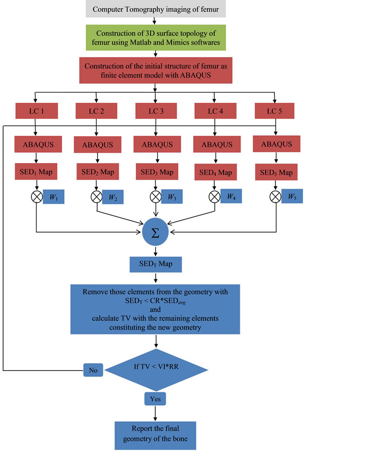
Figure 1. Flowchart of the iterative ESO analysis performed during the study. The parts of the analysis carried out with ABAQUS are indicated by boxes colored in red. The blue colored boxes indicate the post processing carried out using Fortran code. The acronyms are as follows; LC: load cases described as boundary condition on the model, ABAQUS: finite element modelling with qsub routine of ABAQUS, SED: strain energy density, SEDavg: average strain energy density over all elements of updated structure, CR: convergence ratio and set to be 0.001, TV: total volume, VI: initial volume and RR: rejection ratio set to be 0.5 for stopping the iterations when 50% of the total volume is eliminated from the initial design. The parameters (W1, W2, W3, W4, W5) are weight factors associated with the five loading conditions on the femur and were set to (0.35, 0.19, 0.25, 0.15, 0.06) based on a previous publication [9] .

Figure 2. Variation of the average HU values with slice location along the femur shaft as calculated from the cortical sections of the axial CT images.
density maximized on the mid shaft which is known to bear the highest bending load [9] [10] . The sheep femur also has the highest presence of plexiform (stiffer) tissue at the mid shaft as compared to osteonal (weaker) bone [11] . The average value of the HU readings was then calculated from the total cross section that corresponded to the cortical bone at the middle segment of the shaft, and converted to mean bone density and then reinterpreted as elastic modulus using phantom mapping function [12] . The average elastic modulus was estimated from the anterior cortex of the bone as 35 GPa, which was close to the value reported for plexiform bone in the past [13] .
2.3. Extracting the 3D Surface Topology of Femur
The masked images were further processed using Mimics software (Materialise, Leuven, Belgium). The surface boundary of the femur was extracted for the FE modeling.
2.4. Construction of the FE Model of Femur
To numerically simulate the sheep femur, a FE model was created using ABAQUS by following the procedures described previously [14] . The 3D topology of the bone was inputted into ABAQUS and the whole inner volume of the bone was filled completely and uniformly with a tetrahedron mesh of average edge length 2 mm. But for the purpose of comparing the mesh convergence behavior under different element size during the iterations, another model was built with tetrahedrons having an average edge length of 3 mm. For a given discretization, the measured elastic modulus of 35 GPa was assigned to each element. The resulting FE model constituted the initial homogeneous design of the femur, as shown in Figure 3. This construct was later subjected to remodeling under different loads applied externally, as described next.
2.5. Specific Conditions of Mechanical Loading on Numerically Simulated Femur
Characteristics of the musculoskeletal forces acting on the sheep femur have been identified previously with the phases of coherently varying walking cycle [15] [16] . Gait analysis performed on a healthy sheep indicated that on the average, about 62% of the normal walking cycle of sheep reported to be stance and the rest 38% considered to be swing, but contributions of these forces to swing or stance are not equal [9] . The major forms of weight bearing loads experienced by sheep femur in real life physical activity were classified as:
1) Dominant compression on femur head2) Heel-strike3) One-legged stance4) Toe-off and 5) Fall on the hip with impact on the lateral greater trochanter.
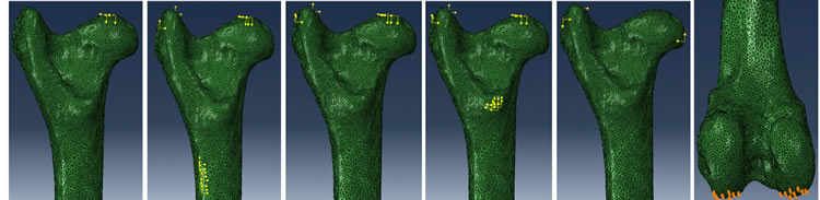
The muscle names exerting these loads on the femur were summarized in Table 1. The locations where the forces acting on the femur were marked by the black dots in Figure 3 and their vectorial representations were displayed schematically in Figure 4. The load magnitudes and directions as well as the target locations were given in Table 2 and Table 3. The values in the tables were determined from previous publications describing the biomechanical forces of the sheep hip joint [9] [15] . At its distal end, the femur was pinned down or mechanically fixed on its condyles (Figure 4(f)).
In this study, we applied the above multiple loading cases and investigated the structural response of the numerically simulated femur using iterative ESO algorithm. The inequal contribution of each load to the normal walking was accounted for by appropriately assigning weight factors that were calculated from the gait analysis of clinically healthy sheep [9] . Our approach was implemented in-house using Fortran software platform and explained next.
2.6. Topology Optimization or Element Removal Criteria
ESO is an iterative method for optimization, where the elements of the FE model are removed from or add to the initial design of structural based on certain criteria at each step. One of the criteria commonly used for the removal of an element is lower strain energy density (SED). To apply this strategy, as shown in Figure 1, we started the optimization process by describing an initial design with a load distribution on the boundary of the
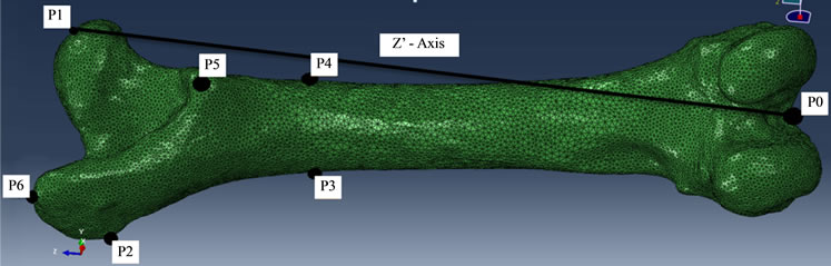
Figure 3. Schematic of the initial FE model of sheep (left side) femur meshed with tetrahedrons with average 2 mm edge size. The marked black points indicate mechanical loading (or boundary condition) applied by muscles on the bone. Black line is the indicator of musculoskeletal coordinate axis (Z’). Note that this initial design was completely filled with uniform elastic young modulus of 35 GPa within its boundary.

Table 1. Muscle names and their attachment points to the femur as indicated by the black dots in Figure 3.
Data adopted from [9] [15] [32] .
 (a) (b) (c) (d) (e) (f)
Figure 4. Five different load cases applied to the simulated bone under normal walking. (a) Fully compressed; (b) Heel strike; (c) Stance; (d) Toe off; (e) Fall and (f) The condyles encastered.
Table 2. Representations of forces in Figure 4 as unit vectors.
Data collected/adopted from [15] [33] [34] .
Table 3. Multiplication coefficients for the unit vectors in Table 2 to account for the body weight of sheep, which was assumed to be 56 Kg (549.4 N).
Data collected/adopted from [9] .
femur and performed iterations until the desired volume of final structure is reached. The optimization problem describing such operation can be formulated as
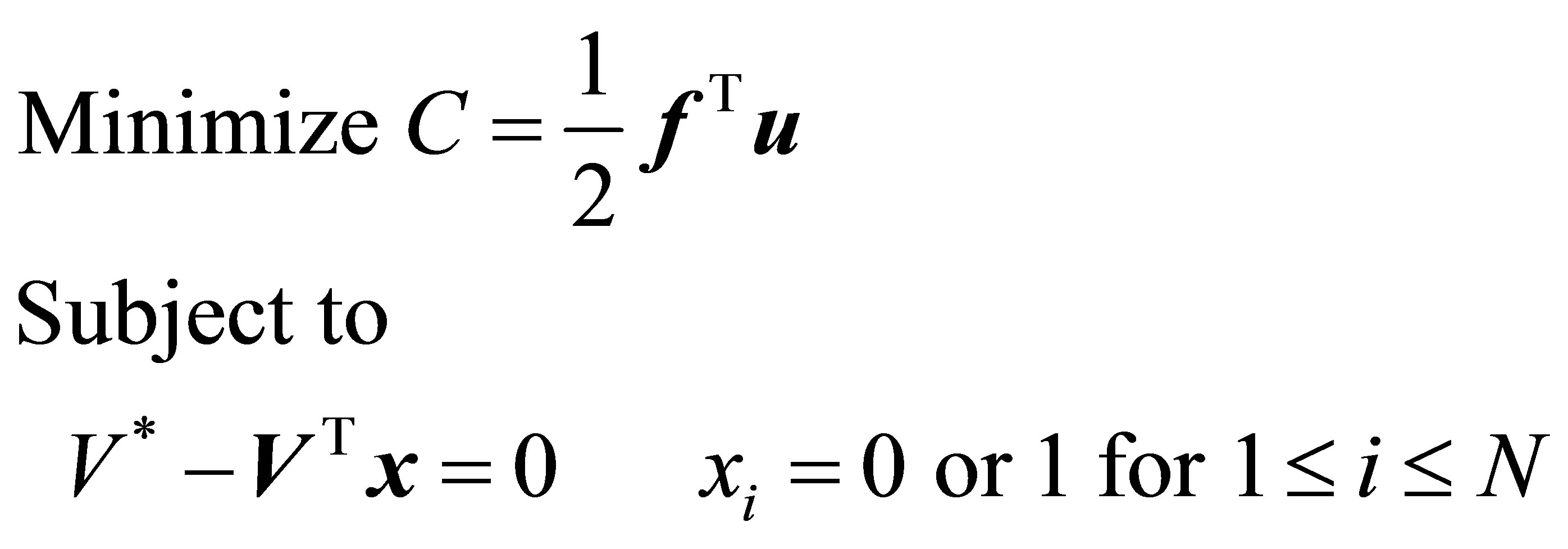 . (1)
. (1)
Here f and u are N dimensional vectors. N denotes number of elements in the initial design. f describes the external load acting on the FE model and u is the nodal displacement. C is the overall compliance. V* is the prescribed total volume of the final structure. Vi is the volume of individual element and xi assumes a binary value, where 1 indicates presence and 0 denotes absence of the underlying element in the structure. The contribution of each loading case was weighted in by a multiplication factor W. For the five loading conditions on the femur in Table 1, the weighting factors were respectively derived from the literature based on the active action time of each (0.35, 0.19, 0.25, 0.15, 0.06) [9] . Normalized SED of an element is defined as half of stress multiplied by strain divided by the volume of the element. When SED in an element was found to attain a relatively low value compared to the other elements during the process, such an element was considered inefficient in supporting the load and hence removed. In addition, the optimization protocol implemented in this study allowed the desired volume of interest to be set 50% of the volume of the initial design. Element erosion was allowed at the shaft region, but restricted at the proximal and distal ends of the femur.
2.7. Muscle Malfunction Effects on Bone Remodelling
The presence of muscle injury or malfunction influences the course of bone remodeling. To study such effects, the force of gluteus medius (applied to P6) or adductor longus (applied to P4) was reduced to 10% of their initial magnitudes. Under each change, ESO was performed. The results with the altered force distribution were presented, compared against that of the healthy bone and discussed to gather insights into the bone remodeling and potential risk of bone fracture following muscle malfunction.
3. Results
The characteristic features of the FE models constructed as the initial designs with two different sizes of tetrahedrons were summarized in Table 4. For the model with finer mesh consisting of average 2 mm edge length elements, both the number of nodes and elements were significantly higher than the model with coarser mesh consisting of average 3 mm element edges. But, the volumes of femur in both models were comparable to the volume 152,326 mm3 estimated from the CT data. Running the ESO procedure in Figure 1 for 128 iterations took about 19 hours and 16 hours for the finer and coarser mesh models, respectively (Table 5).
For both cases, the ESO process converged to meaningful solutions. The convergence rates and behaviors of the iterations were similar to those reported in the previous topology optimization studies [17] . Such outcomes were no surprise because ESO method is known to be mesh independent [17] [18] .
The model with the smaller average 2 mm length edge provided higher resolution output which is presented in the following. Figure 5 shows the femur designs obtained at iterations 5 and 50 of the ESO procedure described in Figure 1. As seen in Figure 5, confining the optimization to only the shaft portion prevented the element erosion at the proximal and distal ends of the femur.
To demonstrate the evolution of the optimization, three locations were selected along the femur in Figure 6 and the femur was viewed from the proximal to distal direction while producing the cross sectional images in Figure 7 at different levels of the iteration. According to the data, the initial design started with a completely filled structure at the 0th iteration.
In the 1st iteration, some elements central to the femur shaft were removed immediately and the element removal was continued in the following iterations. This implied that the innermost elements were the first ones etched away from the model. At the 5th iteration, the shaft has already started looking like a hallow tube. Corollary
Table 4. Features of FE meshes for the initial designs generated with two different sizes of tetrahedrons.
Table 5. Computer run times for two sizes of mesh in ABAQUS.
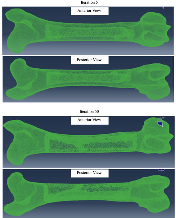
Figure 5. Femur designs at iterations 5 and 50 of the ESO procedure.
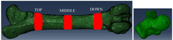
Figure 6. Locations along the femur where the cross sectional images in Figure 7 were produced when the femur was viewed from the proximal to distal direction. The right figure shows the anterior face of the femur.
to this was that the removed elements had the lowest SED values and played minor role in supporting the load acting on the femur.
With further iteration, the elements internal to the bone continued to erode while the elements closer to the femur surface remained intact. The degree of erosion assumed a form that was circumferentially non-uniform and reflected the spatial distribution of the SED with angle. For example, at the 50th iteration, the shaft around
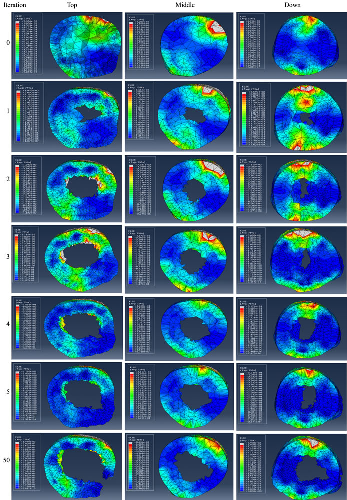
Figure 7. Cross sectional visualization of the remodelled femur at the top, middle and down sections when viewed from the proximal to distal direction at different iterations of the ESO procedure. Color coding is nodal representation of total elastic strain energy in each element, as calculated by routine ELSE in ABAQUS.
the 4 and 10 o’clock regions consisted of inefficient elements. Some regions become completely clear of the elements. Such a case was physically unrealistic, but served the purpose of demonstrating the inherently weak regions of the simulated femur. In real situations, this type of remodeling would have the consequences of weak areas being populated by softer bone tissues.
The CT images in Figure 8 shows the cross sections of the real femur at the locations where the simulated images in Figure 7 were produced. The data in Figure 8 confirmed the trends predicted by the analysis of the bone formation and remodeling with the ESO method in Figure 7.
Figures 9 and 10 show the results of reducing either gluteus medius or adductor longus forces to 10% of the initial magnitudes used for the healthy bone simulations. The results illustrate the shapes and SED distributions of the initial design (at 0th iteration) and the design at an iteration that had a total volume closest to that of the previous healthy femur at the 50th iteration.
4. Discussion
Wolff law suggests that healthy bone would adapt to the loads under which it is placed [19] [20] . In response to an increased load, the bone becomes tougher and thicker to maintain the stress induced within. The inverse of this scenario also holds. In the past studies, this view was checked and its validity was confirmed to a degree

Figure 8. CT images showing the cross sections of the real femur at the locations where the simulated images in Figure 7 were produced.
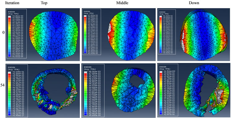
Figure 9. Effect of reducing gluteus medius force on bone remodelling.
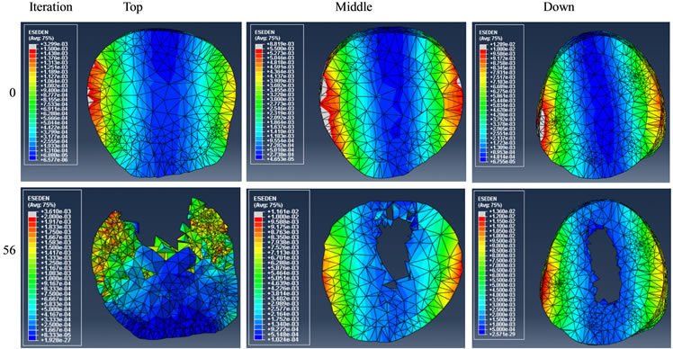
Figure 10. Effect of reducing adductor longus force on bone remodelling.
using numerical analysis [21] [22] . But, since then, the field has progressed and new tools have been developed for analyzing mechanical structures. ESO is one of these tools and was originally proposed for engineering applications involving topology optimization. The approach was originally based on a simple concept of gradually removing inefficient (or extra) material from the initial design of structure which may greatly enhance the performance of the structure [23] [24] . In this study, we employed ESO to numerically investigate the remodeling of femur formation in sheep under normal patterns of mechanical loading exerted during normal walk by the muscles attached to it. We took a macroscopic view and used a simplified approach in modeling the femur. Our efforts led to the implementation of the iterative ESO algorithm in Figure 1 and construction of a numerically simulated femur in Figure 3. One of the simplifications involved filling the whole bone with uniform material properties estimated from CT images (Figure 2). Starting with this design and the combination of the most common loads described in Figure 4 and featured in Tables 1-3, each step of the algorithm was run iteratively and spatially inefficient sections of the bone were revealed and removed, in reality, however, these sections of the bone would not be removed, instead according to Wolff’s view, the tissue type would change from plexiform to mechanically inferior haversian tissue due to the presence of lower mechanical stiffness. Such a change has been reported for the sheep femur, where the posterior femur mostly remodels to harversian tissue type and the anterior part remains lamellar plexiform while the sheep is transforming from young to mature [11] [13] [19] [22] . The presence of the two tissue types with different stiffness around the circumference of the femur may be the result of the mechanical stimulus acting at macroscale [25] . The element removal in Figure 7 was in line with the mechanical principles of Wolff which is confirmed by the design principle of the process of ESO implemented in this study.
Predicting the mechanical properties, failure and risk of bone fracture non-invasively is an active area of research [26] [27] . Any proposed model must be able to predict the strength and strain distribution accurately under different loading conditions. According to the literature, automatic CT-based FE model is typically used for evaluating the acceptability of the mechanical behavior of bone under loading [28] [29] . This study used automatic mesh generation using CT images. Although the study goal was to answer the question of whether the bone formation in real femur would follow the prediction by ESO, our work was also fundamentally a comparative study and can be extended to perform failure and risk analysis of the bone for a given set of both material and geometrical properties using ESO.
Predicting the risk of fracture and failure has been studied on CT based FE models [30] . Muscle malfunction may result in bone remodelling in a specific section due to changes in the mechanical stimulus. By reducing the gluteus medius force, we found that a large portion of anterior and posterior elements were removed and these sections became thinner, as shown in Figure 9. This could be due to the fact that the gluteus medius force trajectories had an opposite effect in comparison with the joint force on the femur head. By this reduction, the joint force must have become dominant which resulted in the preservation of medial/lateral elements and the removal of anterior/posterior elements, thus leading to a higher fracture risk in those thinner areas. On the other hand, the adductor longus connects the medial part of femur to pelvis (on point P4 in Figure 3) with the force pushing from anterior to posterior in adduction. By reducing this muscle force, anterior elements were removed, particularly in the top section, as shown in Figure 10. It is likely that the risk of fracture in the anterior area would have been increased in this scenario of muscle malfunction.
Our analysis considered the femur being loaded statically by only major muscle groups, as such was the case in previous publications [12] [26] [31] . The distal end of the femur was stabilized, rather than loaded by the muscles or tendons attached to this end. These may be viewed as limitations of this study because it lacked dynamic or cyclic loading as well as inclusion of the other loadings.
In FE modeling, the spatial dependence of the elasticity variation was not taken into consideration at the design and whole femur was assigned a constant elastic modulus corresponding to the plexiform bone. This assignment remained the same during the iterations of the optimization algorithm. However, heterogeneous, instead of homogenous elastic modulus values assigned to smaller finite elements could have made the model better mimic the real femur.
5. Conclusion
CT images of femur can be used to measure the femur’s elastic properties and to construct finite element model of the femur. It may be feasible to apply ESO to problems in biomechanics to understand the structural remodeling of biological tissue formation, such as bone, under mechanical loading. Performing ESO on numerically simulated femur with an initial design consisting of stiffest plexiform tissue can help recognize the bone regions that can be replaced with less stiff ostoenal tissue to represent the process of remodeling according to the mechanical stimulus. Hence, such simulations can provide insights on whether the material distribution has been assigned in a mechanically optimized fashion to the femur topology or to determine those sections that are eligible for being attributed lower stiffness to carry the internal stress. Such findings highlight the existence of mechanically optimum relationship between the topology and stiffness, and overall can be used to confirm the Wolff’s law of bone transformation where the tissue types are distributed in mechanically optimum fashion to counteract the applied forces. The ESO simulations may also provide useful insight into the risk of bone fracture as a result of muscle malfunction.
References
- Fan, Y., et al. (2011) Optimal Principle of Bone Structure. PLoS One, 6, e28868. http://dx.doi.org/10.1371/journal.pone.0028868
- Bouguecha, A., Weigel, N., Behrens, B.-A., Stukenborg-Colsman, C. and Waizy, H. (2011) Numerical Simulation of Strain-Adaptive Bone Remodelling in the Ankle Joint. BioMedical Engineering OnLine, 10, 1-13. http://dx.doi.org/10.1186/1475-925X-10-58
- Comiskey, D.P., MacDonald, B.J., McCartney, W.T., Synnott, K. and O’Byrne, J. (2012) Predicting the External Formation of a Bone Fracture Callus: An Optimisation Approach. Computer Methods in Biomechanics and Biomedical Engineering, 15, 779-785. http://dx.doi.org/10.1080/10255842.2011.560843
- Comiskey, D., MacDonald, B.J., McCartney, W.T., Synnott, K. and O’Byrne, J. (2013) Predicting the External Formation of Callus Tissues in Oblique Bone Fractures: Idealised and Clinical Case Studies. Biomechanics and Modeling in Mechanobiology, 12, 1277-1282. http://dx.doi.org/10.1007/s10237-012-0468-6
- Schulte, F.A., et al. (2013) Local Mechanical Stimuli Regulate Bone Formation and Resorption in Mice at the Tissue Level. PLoS One, 8, e62172. http://dx.doi.org/10.1371/journal.pone.0062172
- Xie, Y.M. and Steven, G.P. (1993) A Simple Evolutionary Procedure for Structural Optimization. Computers & Structures, 49, 885-896. http://dx.doi.org/10.1016/0045-7949(93)90035-C
- Hangartner, T.N. and Overton, T.R. (1982) Quantitative Measurement of Bone Density Using Gamma-Ray Computed Tomography. Journal of Computer Assisted Tomography, 6, 1156-1162. http://dx.doi.org/10.1097/00004728-198212000-00017
- Latifi, M.H., et al. (2012) Prospects of Implant with Locking Plate in Fixation of Subtrochanteric Fracture: Experimental Demonstration of Its Potential Benefits on Synthetic Femur Model with Supportive Hierarchical Nonlinear Hyperelastic Finite Element Analysis. BioMedical Engineering OnLine, 11, 1-18.
- Agostinho, F., et al. (2012) Gait Analysis in Clinically Healthy Sheep from Three Different Age Groups Using a Pressure-Sensitive Walkway. BMC Veterinary Research, 8, 87-94. http://dx.doi.org/10.1186/1746-6148-8-87
- Bramer, J.A., et al. (1998) Representative Assessment of Long Bone Shaft Biomechanical Properties: An Optimized Testing Method. Journal of Biomechanics, 31, 741-745. http://dx.doi.org/10.1016/S0021-9290(98)00101-8
- Yamato, Y., Matsukawa, M., Otani, T., Yamazaki, K. and Nagano, A. (2006) Distribution of Longitudinal Wave Properties in Bovine Cortical Bone in Vitro. Ultrasonics, 44, e233-e237.
- Yosibash, Z., Padan, R., Joskowicz, L. and Milgrom, C. (2007) A CT-Based High-Order Finite Element Analysis of the Human Proximal Femur Compared to in-Vitro Experiments. Journal of Biomechanical Engineering-Transactions of the Asme, 129, 297-309. http://dx.doi.org/10.1115/1.2720906
- Katz, L.J., et al. (1984) The Effects of Remodeling on the Elastic Properties of Bone. Calcified Tissue International, 36, S31-S36. http://dx.doi.org/10.1007/BF02406131
- Tomaszewski, P.K., Verdonschot, N., Bulstra, S.K. and Verkerke, G.J. (2010) A Comparative Finite-Element Analysis of Bone Failure and Load Transfer of Osseointegrated Prostheses Fixations. Annals of Biomedical Engineering, 38, 2418-2427. http://dx.doi.org/10.1007/s10439-010-9966-9
- Bergmann, G., Graichen, F. and Rohlmann, A. (1999) Hip Joint Forces in Sheep. Journal of Biomechanics, 32, 769- 777. http://dx.doi.org/10.1016/S0021-9290(99)00068-8
- Orth, P. and Madry, H. (2013) A Low Morbidity Surgical Approach to the Sheep Femoral Trochlea. Bmc Musculoskeletal Disorders, 14, 5. http://dx.doi.org/10.1186/1471-2474-14-5
- Cho, K.H., Park, J.Y., Ryu, S.P. and Han, S.Y. (2011) Reliability-Based Topology Optimization Based on Bidirectional Evolutionary Structural Optimization Using Multi-Objective Sensitivity Numbers. International Journal of Automotive Technology, 12, 849-856. http://dx.doi.org/10.1007/s12239-011-0097-6
- Huang, X. and Xie, Y.M. (2007) Convergent and Mesh-Independent Solutions for the Bi-Directional Evolutionary Structural Optimization Method. Finite Elements in Analysis and Design, 43, 1039-1049. http://dx.doi.org/10.1016/j.finel.2007.06.006
- Petit, M.A., et al. (2008) Proximal Femur Mechanical Adaptation to Weight Gain in Late Adolescence: A Six-Year Longitudinal Study. Journal of Bone and Mineral Research, 23, 180-188. http://dx.doi.org/10.1359/jbmr.071018
- Seeman, E. (2008) Bone Quality: The Material and Structural Basis of Bone Strength. Journal of Bone and Mineral Metabolism, 26, 1-8. http://dx.doi.org/10.1007/s00774-007-0793-5
- Boyle, C. and Kim, I.Y. (2011) Three-Dimensional Micro-Level Computational Study of Wolff’s Law via Trabecular Bone Remodeling in the Human Proximal Femur Using Design Space Topology Optimization. Journal of Biomechanics, 44, 935-942. http://dx.doi.org/10.1016/j.jbiomech.2010.11.029
- Robling Ag Fau-Castillo, A.B., Castillo Ab Fau-Turner, C.H. and Turner, C.H. (2006) Biomechanical and Molecular Regulation of Bone Remodeling. Annual Review of Biomedical Engineering, 8, 455-498.
- Huang, X. and Xie, Y.M. (2009) Bi-Directional Evolutionary Topology Optimization of Continuum Structures with One or Multiple Materials. Computational Mechanics, 43, 393-401. http://dx.doi.org/10.1007/s00466-008-0312-0
- Woon, S.Y., Tong, L., Querin, O.M. and Steven, G.P. (2005) Effective Optimisation of Continuum Topologies through a Multi-GA System. Computer Methods in Applied Mechanics and Engineering, 194, 3416-3437. http://dx.doi.org/10.1016/j.cma.2004.12.025
- Machado, M.M., Fernandes, P.R., Cardadeiro, G. and Baptista, F. (2013) Femoral Neck Bone Adaptation to WeightBearing Physical Activity by Computational Analysis. Journal of Biomechanics, 46, 2179-2185. http://dx.doi.org/10.1016/j.jbiomech.2013.06.031
- R. A. Horch, D. F. Gochberg, J. S. Nyman and M. D. Does, “Non-invasive predictors of human cortical bone mechanical properties: T-2-Discriminated H-1 NMR compared with high resolution X-ray,” PLoS ONE, Vol. 6, No. 1, 2011, p. e16359. http://dx.doi.org/10.1371/journal.pone.0016359
- Müller, R. and Rüegsegger, P. (1995) Three-Dimensional Finite Element Modelling of Non-Invasively Assessed Trabecular Bone Structures. Medical Engineering & Physics, 17, 126-133. http://dx.doi.org/10.1016/1350-4533(95)91884-J
- Cristofolini, L., et al. (2010) Mechanical Testing of Bones: The Positive Synergy of Finite-Element Models and in Vitro Experiments. Philosophical Transactions of the Royal Society A: Mathematical Physical and Engineering Sciences, 368, 2725-2763.
- Kim, H.S., et al. (2012) Finite Element Modeling Technique for Predicting Mechanical Behaviors on Mandible Bone during Mastication. Journal of Advanced Prosthodontics, 4, 218-226. http://dx.doi.org/10.4047/jap.2012.4.4.218
- Keyak, J.H., Rossi, S.A., Jones, K.A. and Skinner, H.B. (1998) Prediction of Femoral Fracture Load Using Automated Finite Element Modeling. Journal of Biomechanics, 31, 125-133. http://dx.doi.org/10.1016/S0021-9290(97)00123-1
- Silva, M.J., Keaveny, T.M. and Hayes, W.C. (1998) Computed Tomography-Based Finite Element Analysis Predicts Failure Loads and Fracture Patterns for Vertebral Sections. Journal of Orthopaedic Research, 16, 300-308. http://dx.doi.org/10.1002/jor.1100160305
- Hutzschenreuter, P.O., Sekler, E. and Faust, G. (1993) Loads on Muscles, Tendons and Bones in the Hind Extremities of Sheep—A Theoretical Study. Anatomia Histologia Embryologia—Journal of Veterinary Medicine Series C-Zentralblatt fur Veterinarmedizin Reihe C, 22, 67-82.
- Fraysse, F., et al. (2009) Comparison of Global and Joint-to-Joint Methods for Estimating the Hip Joint Load and the Muscle Forces during Walking. Journal of Biomechanics, 42, 2357-2362.
- Page, A.E., et al. (1993) Determination of Loading Parameters in the Canine Hip in Vivo. Journal of Biomechanics, 26, 571-579.