Intelligent Control and Automation
Vol.10 No.01(2019), Article ID:90829,33 pages
10.4236/ica.2019.101002
Tensor-Centric Warfare V: Topology of Systems Confrontation
Vladimir Ivancevic1, Peyam Pourbeik2, Darryn Reid1
1Joint and Operations Analysis Division, Defence Science & Technology Group, Canberra, Australia
2Cyber and Electronic Warfare Division, Defence Science & Technology Group, Canberra, Australia

Copyright © 2019 by author(s) and Scientific Research Publishing Inc.
This work is licensed under the Creative Commons Attribution International License (CC BY 4.0).
http://creativecommons.org/licenses/by/4.0/


Received: January 22, 2019; Accepted: February 25, 2019; Published: February 28, 2019
ABSTRACT
In this paper, as a new contribution to the tensor-centric warfare (TCW) series [1] [2] [3] [4], we extend the kinetic TCW-framework to include non-kinetic effects, by addressing a general systems confrontation [5], which is waged not only in the traditional physical Air-Land-Sea domains, but also simultaneously across multiple non-physical domains, including cyberspace and social networks. Upon this basis, this paper attempts to address a more general analytical scenario using rigorous topological methods to introduce a two-level topological representation of modern armed conflict; in doing so, it extends from the traditional red-blue model of conflict to a red-blue-green model, where green represents various neutral elements as active factions; indeed, green can effectively decide the outcomes from red-blue conflict. System confrontations at various stages of the scenario will be defined by the non-equilibrium phase transitions which are superficially characterized by sudden entropy growth. These will be shown to have the underlying topology changes of the systems-battlespace. The two-level topological analysis of the systems-battlespace is utilized to address the question of topology changes in the combined battlespace. Once an intuitive analysis of the combined battlespace topology is performed, a rigorous topological analysis follows using (co)homological invariants of the combined systems-battlespace manifold.
Keywords:
Tensor-Centric Warfare, Systems Confrontation, Systems-Battlespace Topology, Cobordisms and Morse Functions, Morse-Smale Homology, Morse-Witten Cohomology, Hodge-De Rham Theory

1. Introduction
The principal objective of the Modeling Complex Warfighting (MCW) Strategic Research Investment (SRI) is to better enable dealing with uncertainty, meaning achieving reliable decision-making in environments that are non-ergodic. Such systems are incomprehensible, in a sense, through observation of past data, because they lack stability and manifest unique transient states. Phenomena associated with war and battle are inherently non-ergodic, a fact that has been observed at least since the birth of modern military thinking (see, for instance, [6] and references therein1). This paper attempts to approach the MCW problem from the multilayered nature of warfare and look at Blue, Red and Green entities. The aim is to undertake analysis which closely represents the realities of modern warfare. When modeling complex modern combined battlefields it is therefore important to consider neutral forces―which we label “Green”―since they are much more now than in the past even the central feature of the strategic situation. Indeed, in modern asymmetric confrontations neutral or non-engaging groups have been known to side with one side or the other or even to engage actively in conflict, which rapidly changes the dynamics of the situation. Hence, social and psychological domains play an increasingly significant role in understanding the dynamics of modern armed conflict.
The dynamics of the combined effects of these and other factors mean that the statistical properties of such problem environments are non-stationary. As a result, the outcomes of battles are not predictable, since the battle is inherently non-ergodic; yet, it is possible to deal with such systems nonetheless by establishing conditions that are weaker than ergodicity, which have essentially topology-changing nature.
The tensor-centric warfare (TCW) series of papers (see [1] [2] [3] [4]) have established a basis for MCW to investigate uncertainty in modern war and battle, using entropic dynamical properties in place of statistical predictions about future outcomes. More specifically, the TCW framework has proposed the following pair of Red-vs-Blue tensorial combat models (formally, the pair of Red-Blue vectorfields; their solution for some initial conditions gives the pair of Red-Blue flows):
(1)
where and the Red and Blue forces are defined as vectors and , defined on their respective configuration n-manifolds (with local coordinates , for ) and (with local coordinates ). The Red and Blue vectorfields, and , include the following terms (placed on the right-hand side of Equation (1)):
• Linear Lanchester-type terms, and , with combat tensors and defined via bipartite and tripartite adjacency matrices, respectively defining Red and Blue aircraft formations (according to the aircraft-combat scenario from [1] [12]);
• Quadratic Lanchester-type terms, and , with the 4th-order tensors and representing strategic, tactical and operational capabilities of the Red and Blue forces (see [1]);
• Entropic Lie-dragging of the opposite side terms, and , where and . In case of resistance, the Lie derivatives are positive, and , so that the non-equilibrium battlefield entropy grows, ; in case of non-resistance, the Lie derivatives vanish, and , so that the battlefield entropy is conserved, (see [2]);
• Entropic Red-Blue commutators, and , for modeling warfare symmetry (see [2]), in which the entropy grows in the asymmetric case (>0) and stays conserved in the symmetric case (=0);
• Hamilton-Langevin delta strikes, and , including (on both sides) discrete striking spectra (slow-fire missiles) and continuous striking spectra (rapid-fire missiles), as well as bidirectional random strikes, Hamiltonian vectorfields, self-dissipation, opponent-caused dissipation and non-delta random forces (see [3] for the full explanation of all included temporally-confined kinetic strike/missile terms).
In the present paper, we extend the above kinetic Red-Blue framework to include non-kinetic effects, by addressing the general systems-confrontation [5], which is waged not only in the traditional physical Air-Land-Sea domains, but also in modern non-physical environments, such as cyberspace, electromagnetic spectrum, psychological and social network domains. This paper attempts to address this complex contemporary warfare situation using rigorous methods and techniques from modern algebraic topology; specifically, by extending the kinetic Red-Blue scenario (Figure 1) into more general and more representative kinetic + non-kinetic Red-Blue-Green scenarios (Figure 2).
Dynamically speaking, the basic Red-Blue pair of vectorfields (1) is extended with the following Green vectorfield:
(2)

Figure 1. Sketch of the Red-Blue battlespace cobordism: the combined Red-Blue battlespace -manifold W has the N-dimensional boundary that is defined as the disjoint union of the Red and Blue configuration N-manifolds, and , formally given by: . The combined battlespace manifold W defines the equivalence class of cobordisms, , between the Red and Blue manifolds. See section 2 for technical details.

Figure 2. Sketch of the Red-Blue-Green systems-battlespace cobordism , addressing a general systems-confrontation scenario, in which the non-kinetic effects are embedded in the Green manifold. The combined battlespace manifold W now defines the equivalence class of cobordisms, , between the Red, Blue and Green manifolds. See Section 2 for technical details.
where is the Green flow on the Green manifold ; and represent non-kinetic effects in scalar and vector form, respectively, and all the other terms are the same as in Equation (1). Notice that on the right-hand side of Equation (2) al the tensors are the sums of the corresponding Red and Blue tensors. This insures the fact that the Green force includes both Red and Blue forces and the covariance is preserved. Also, the kinetic delta strikes are missing, which gives the highest importance to entropic Lie-dragging ( , with or without resistance) of the Red-and-Blue cyberspace, electromagnetic, psychological and social-network domains (encaptured in the tensors and ).
Topological motivation for the present paper is inherited from the influence on modern physics by John Wheeler from Princeton2. Although we might have some well-defined and (numerically) solvable local TCW Equations (1)-(2), we lack a picture of the global topology of the systems-battlespace-the environmental configuration manifold in which the combat happens-with its dramatic spacial (eliptic/hyperbolic) changes. In (1) both the Red and Blue vectorfields, and , and their corresponding flows, and , which consist of the integral lines of the vectorfields and obtained by their numerical integration starting from the chosen initial conditions, and , respectively-are defined on their respective configuration n-manifolds3, and . To give the global picture of the battlefields governed by local Equation (1)-(2) we need to perform the topological analysis of the joint manifold including all three submanifolds: , and .
Global topological analysis is an extension of local geometric analysis. To utilize the geometric framework most suitable for the present topological analysis4, we will assume that Red and Blue (as well as Green) configuration manifolds, , and , are endowed with the pseudo-Riemannian geometry, which is both elliptic (positive metric) and hyperbolic (negative metric; see, e.g. [7] [8]), defined by their corresponding quadratic forms, , and . These three quadratic forms are not necessarily positive-definite, which would be the necessary condition for the strict Riemannian geometry, but only non-degenerate, which is a weaker condition. Since we are working in the more general pseudo-Riemannian geometry framework, the three quadratic forms, , and , can be either positive or negative, depending on their respective combat tensors, , and , which have initially been defined as combinations of kink (Tanh) and bell (Sech) functions applied to the bipartite-Red and tripartite-Blue adjacency matrices from the initial scenario5 from [1] [12] (as depicted in Figure 1). This gives us the level of generality needed for a reasonable representation of the systems-battlespace, but can be easily generalized further to the system confrontation level by adding non-kinetic terms, mostly present within the combined Green tensor: .
The non-equilibrium phase transitions occurring at the battlefield at various stages of warfare, can be superficially characterized by sudden entropy growth. However, these rapid changes of the systems-battlespace always have underlying structural topology changes (see [13] and the references therein). In this paper, we give a two-level topological analysis of the systems-battlespace. We start visually by giving a largely intuitive analysis of the systems-battlespace topology using Thom’s cobordisms and Morse functions. Then we move into a rigorous topological analysis of the systems-battlespace by deriving its (co)homological invariants, which can be summarized by the famous dictum of John Wheeler: “The boundary of a boundary is zero (BBZ)”. Specifically, we derive the Morse-Smale homology and the Morse-Witten cohomology of the systems-battlespace manifold. All the necessary geometrical and topological background is given in the self-content and comprehensive Appendix, which provides the Hodge-de Rham theory based on the Stokes theorem. Then we perform a rigorous analysis of the systems-battlespace topology with its dramatic spatial changes by deriving its (co)homological invariants6.
2. Components of the Systems-Battlespace Topology: Cobordisms and Morse Functions
In this section we develop the basic differential topology of the systems-battlespace, mainly following the work of the Fields medalist John Milnor [15] [16] [17].
2.1. Systems-Battlespace Cobordisms: Red-Blue versus Red-Blue-Green
To start with the systems-battlespace topology, we introduce an important concept from differential topology (and its gravitational-physics applications): the so-called cobordism7. Briefly, the cobordism relation, denoted , between two compact (i.e., closed and bounded) n-manifolds, and , means that their disjoint union is the boundary of a compact -manifold W. In other words, cobordism between two compact n-manifolds and is the compact -manifold W whose boundary is the disjoint union of and . This is an equivalence relation and the equivalence class of cobordisms is denoted by 8 (for technical details, see e.g. [7] [8] [17] [18]). In our case, the Red-Blue systems-battlespace -manifold W has the nD boundary (see Figure 1), and the equivalence class of systems-battlespace cobordisms given by:
The two-party battlespace cobordism from Figure 1 can be extended into a three-party systems-battlespace manifold , depicted in Figure 2, as follows. We introduce the composition of cobordisms, , which can be defined in case of a triple manifold, , so that the glued cobordism, , where represents the gluing operation, is defined by the following (semigroup-like operation) map9:
which in our case of an extended three-party systems-battlespace manifold, , reads:
In the language of abstract algebra, we say that the following diagram commutes:

In plain English, this commutative diagram reads: if we have a cobordism between the Red and Blue manifolds, and a cobordism between the Blue and Green manifolds, then we also have a cobordism between the (initial) Red and (final) Green manifolds. That is, (see Figure 2).
Clearly, this operation can be extended to any number of parties, producing the so-called chain cobordism, between the first and the last manifold; e.g., in case of four parties/manifolds (Red, Blue, Green, Yellow), we have the following commutative chain cobordism:
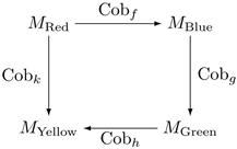
That is, , etc.
2.2. Morse Functions of the Systems-Battlespace: Red-Blue versus Red-Blue-Green
Closely-related to the systems-battlespace cobordisms are the Morse functions of the systems-battlespace. Namely, on the Red-Blue systems-battlespace (Figure 1), which is a pseudo-Riemannian n-manifold:
we can define the real-valued Red-Blue Morse function, (see [15] [16] [17]), as a sum of the two pseudo-Riemannian quadratic forms:
which can be seen as the Red-Blue landscape. Its gradient vectorfield:
according to the Morse lemma, defines the Red-Blue level set10 of equipotential contour lines (of equal altitude) at the critical points p of where the gradient vanishes: . The finite set of m critical points of is denoted by Crit( ).
In addition, we need to consider only nondegenerate critical points of , that is, only those critical points p of the vanishing gradient, , which have the nondegenerate Hessian or, non-singular Hessian matrix:
By definition, the function is Morse if all critical points are nondegenerate. All nondegenerate critical points in Crit( ) are isolated in the Red-Blue systems-battlespace W.
The index of each critical point p is the number of negative eigenvalues of the Hessian matrix . In other words, each critical point p of the Red-Blue Morse function has its own index , which is the number of independent directions around p in which decreases. Therefore, we have natural indices of for the minima of , for the saddles of , and for the maxima of .
Topology change of the Red-Blue systems-battlespace happens as an abrupt change of the shape of the level sets of the Morse function whenever it passes through the critical values where , otherwise the topology of W does not change. The mechanism of topology change is attaching a -cell (the so-called “handlebody”) to , completely determined by the index , at the critical points p of . Therefore, the index determines the topology changes of the Red-Blue systems-battlespace W (from Figure 1)11.
According to the Morse-cobordism theorem (see [15] [16] [17]), the Red-Blue Morse function has a finite number of critical points of index , and every cobordism has its Morse function, characterized by the Morse number of a cobordism12, .
The fundamental topological invariant of the Red-Blue systems-battlespace is its Euler characteristic, , defined as the alternating sum of the critical points :
which is equivalent to the alternating sum of the Betti numbers13 of the systems-battlespace W:
Based on the sign of the quadratic forms and , we can distinguish the following four principal cases of the Red-Blue landscape topology, or four critical points, of the Morse function 14, with its corresponding indices15:
Case 1 (depicted in Figure 3): both the Red and Blue quadratic forms are positive, , which gives the global landscape minimum, or the global minimum of the Morse function , with index 0. Its vanishing gradient vectorfield, , defines the level set composed of concentric contour lines.
Case 2 (depicted in Figure 4): the Red quadratic form is positive, , and the Blue quadratic form is negative, , which gives the left landscape saddle (or, mountain passage) in the Red direction, or the saddle-point of the Morse function , with index 1. Its vanishing gradient vectorfield, , defines the Red-saddle level set of contour lines.

Figure 3. Case 1 of the Red-Blue landscape topology: the 3D-plot of the Morse function (left, showing the global surface minimum) and the contour plot of its gradient vectorfield (right, showing the level set). In this case, both the Red and Blue quadratic forms are positive: , the Morse function has index 0, and the vanishing gradient vectorfield, , defines the level set composed of concentric contour lines.

Figure 4. Case 2 of the Red-Blue landscape topology: the 3D-plot of the Morse function (left, showing the Red-saddle) and the contour plot of its gradient vectorfield (right, showing the level set). In this case, the Red quadratic form is positive, , and the Blue quadratic form is negative, , the Morse function has index 1, and the vanishing gradient vectorfield, , defines the Red-saddle level set of contour lines.
Case 3 (depicted in Figure 5): the Red quadratic form is negative, , and the Blue quadratic form is positive, , which gives the right landscape saddle (or, mountain passage) in the Blue direction, or the saddle-point of the Morse function , with index 1. Its vanishing gradient vectorfield, , defines the Blue-saddle level set of contour lines.
Case 4 (depicted in Figure 6): both the Red and Blue quadratic forms are negative, , which gives the global landscape maximum, or the global maximum of the Morse function , with index 2. Its vanishing gradient vectorfield, , defines the level set composed of concentric contour lines.
Now, we can introduce the third player into our wargame, the Green force , represented by its own pseudo-Riemannian quadratic form:

Figure 5. Case 3 of the Red-Blue landscape topology: the 3D-plot of the Morse function (left, showing the Blue-saddle) and the contour plot of its gradient vectorfield (right, showing the level set). In this case, the Red quadratic form is negative, , and the Blue quadratic form is positive, , the Morse function has index 1, and the vanishing gradient vectorfield, , defines the Blue-saddle level set of contour lines.

Figure 6. Case 4 of the Red-Blue landscape topology: the 3D-plot of the Morse function (left, showing the global surface maximum) and the contour plot of its gradient vectorfield (right, showing the level set). In this case, both the Red and Blue quadratic forms are negative, , the Morse function has index 2, and the vanishing gradient vectorfield, , defines the level set composed of concentric contour lines.
where the social-network type, system-confrontation tensor is defined as combinations of kink (Tanh) and bell (Sech) functions applied to Green force adjacency matrix. In this way, we obtain the Red-Blue-Green systems-battlespace , which is also a pseudo-Riemannian -manifold.
On the triple configuration manifold , depicted in Figure 2, we can define the Red-Blue-Green Morse function , as a sum of all three pseudo-Riemannian quadratic forms:
which represents the Red-Blue-Green landscape. Its gradient vectorfield:
according to the Morse lemma, defines the Red-Blue-Green level set16 of equipotential contour lines (see Figure 7) passing through the critical points p of where the gradient vanishes: . The finite set of m critical points of is denoted by Crit( ).
In addition, we need to consider only nondegenerate critical points of , that is, only those critical points p of the vanishing gradient, , which have the nondegenerate Hessian or, non-singular Hessian matrix:
By definition, the function is Morse if its all critical points are nondegenerate. All nondegenerate critical points in Crit( ) are isolated in the Red-Blue systems-battlespace W.

Figure 7. The Red-Blue-Green landscape topology depicted as the 3D contour plots of the Morse function , passing though the critical points p in which the gradient vanishes: : (a) all three quadratic forms have the same sign (either positive or negative)-resulting in elliptic geometry of the Red-Blue-Green landscape; (b) Red and Green forms are positive and Blue is negative, giving hyperbolic geometry of the Red-Blue-Green landscape; (c) Red and Blue are positive and Green is negative, giving hyperbolic geometry of the Red-Blue-Green landscape; (d) Blue and Green are positive and Red is negative, giving hyperbolic geometry of the Red-Blue-Green landscape; all other combinations reduce to these four cases.
As before, the index of each critical point p of the Morse function is the number of negative eigenvalues of the Hessian matrix . Topology change of the Red-Blue-Green systems-battlespace happens as an abrupt change of the shape of the level sets of the Morse function whenever it passes through the critical values where , otherwise the topology of does not change. The mechanism of topology change is attaching a -cell/handlebody, completely determined by the index , at the critical points p of . Therefore, the index determines the topology changes of the Red-Blue-Green systems-battlespace (from Figure 2).
As in the case of cobordisms, this 3-party Morse function can be extended to address more players (e.g., various groups within Green, various coalition partners within Blue and Red, or even a third conflicting Yellow force) in the wargame.
3. Morse (Co)homology of the Systems-Battlespace
In this section, we move to the realm of (co)homology, which can be summarized by Wheeler’s BBZ dictum: “the boundary of a boundary is zero”. We explore the systems-battlespace topology changes, using Morse (co)homology techniques. We will apply Morse (co)homology to the systems-battlespace-cobordism n-manifold W using two approaches, classical approach of Morse homology and modern approach of Morse cohomology (see the Appendix for the basic (co)homology definitions, all rooted in the BBZ dictum).
3.1. Morse-Smale Homology of the Systems-Battlespace
The basic Morse theory was further developed into the Morse homology17 by three Fields Medalists: R. Thom, S. Smale and J. Milnor. In this section we give a brief overview of of Morse homology, applied to the systems-battlespace-cobordism manifold W, using the abbreviated Morse-Smale approach (for a detailed technical review of Morse homology, see [20]).
As a background, we summarize and make the qualitative concepts from the previous section more precise and, for simplicity, restricted to the Red-Blue systems-battlespace. Let represent a -smooth Morse function on the systems-battlespace-cobordism n-manifold W, equipped with the pseudo-Riemannian metric tensor: . The point is the critical point of if . In local coordinates in a neighborhood of on W,
this means for
. The (finite) set of critical points of is denoted by Crit( ). The Hessian of the Morse function at a critical point defines a symmetric bilinear form:
on the tangent space to the systems-battlespace-cobordism manifold at the point , which is in local coordinates represented by the matrix
of second partial derivatives, . Index and nullity of the matrix
are called the index and nullity of the critical point of the Morse function . Since W is a compact n-manifold, it is always possible to alter a given Morse function into a self-indexing Morse function, which has: , for every critical point (for the proof, see [17]).
We develop the Morse homology of the systems-battlespace-cobordism n-manifold W in the following three steps:
1) On the systems-battlespace manifold W we define the negative gradient flow, ( ), as a map such that:
(3)
From the work of Smale [22] [23], it follows that for a generic metric , the corresponding Hessian has only nondegenerate eigenvalues.
2) Using the negative gradient flow (3), we can decompose the systems-battlespace manifold W into a disjoint union of unstable submanifolds,18 , (or equivalently, a disjoint union of stable submanifolds, ), using the prescription due to R. Thom. Let x be a critical point of the Morse function . We define the unstable submanifold, , of the point x under the negative gradient flow ( ), to be the set of all points flowing from the critical point x, formally:
so is an embedded open disk in W with dimension equal to .
Similarly, we define the stable submanifold, , of the point x under the negative gradient flow ( ), to be the set of all points flowing into the critical point x, formally:
so an embedded open disk in W with dimension equal to .
A function is said to be Morse-Smale if the unstable and stable submanifolds intersect transversely for any two critical points, x and y of . Here comes the Morse--Smale condition: for a generic metric the intersection: is transverse19.
1) We can now define the boundary operator (see Appendix A.2), as:
where is the number of points in the quotient manifold: . The proof of the BBZ-condition: is based on gluing and cobordism arguments (see [20]). The corresponding Morse homology group:
states that, for two generic Morse functions , their homology groups and are isomorphic20. Furthermore, for a generic they are isomorphic [17] to the singular homology group (see Appendix A.2) of the systems-battlespace manifold W: .
3.2. Morse-Witten Cohomology of the Systems-Battlespace
Apart from the “classical” Thom-Smale-Milnor approach to Morse homology, in 1980s Ed Witten from Princeton (the only physicist who become the Fields Medalist) rediscovered in [24] the way of computing the cohomology group of an oriented compact Riemannian n-manifold M, in terms of the critical points, Crit(f), of a Morse function , applying the Hodge-de Rham theory (presented in Appendix ).
Witten’s approach (see [24] [25] [26]) is based on the set/group of all harmonic p-forms on M, defined via the Hodge Laplacian as:
Since every harmonic p-form is closed ( ), we have a linear map: , by taking the de Rham cohomology class . The de Rham theorem states that the de Rham cohomology is isomorphic to the singular homology , as well as to any other cohomology with real coefficients, . In addition, the Hodge theorem states that an arbitrary de Rham cohomology class of an oriented compact Riemannian manifold M can be represented by a unique harmonic form , which means that the natural map: is actually an isomorphism: .
We derive the Morse-Witten cohomology for the Red-Blue systems-battlespace cobordism n-manifold W in the following four steps:
1) To start with, we take the Red-Blue Morse function along with the pseudo-Riemannian metric , and consider the long de Rham complex on W (i.e., the long exact sequence of exterior vector-spaces ; see Appendix A.2):
The complex can be decomposed into the direct sum of finite-dimensional eigenspaces of the Hodge Laplacian as:
The Hodge-de Rham theory (see Appendix A.3) implies the following isomorphisms:
2) Next, the very definition of the Hodge Laplacian, , implies that its product with the exterior de Rham differential d (as well as with the codifferential ) is commutative:
Therefore, we can restrict the de Rham differential d to by acting on the subcomplex: , and obtain the -restricted de Rham complex:
To prove that the restricted de Rham complex is exact, we note that if any p-form is in the kernel of , Ker( ), then ; therefore we have:
Since commutes with both d and , we see that ,
which means that the complex is exact. From the exactness of the restricted de Rham complex , it follows that the a-parameterized curve of complexes: has as its cohomology the set/group of all harmonic p-forms on W, for any real .
3) We can now introduce Witten’s main idea from [24] : conjugating the de Rham differential, , by multiplication/composition with (for the Morse function and some real parameter ), gives a deformed closed coboundary operator, , defined by:
(compare with Equations (11)-(12) in Appendix A.3). The deformed differential yields the deformed de Rham cohomology, also called the Witten cohomology:
which is also isomorphic to : because we are only conjugating the de Rham differential d with .
4) The deformed cohomology, , is computed using the Hodge theory, by considering the Witten Laplacian: and the decomposition: , where is the eigenspace of , along with the t-parameterized curve of the chain complexes: , spanned by all eigenforms of with eigenvalues . The t-parameterized curve of the chain complexes: , generated by the Witten Laplacian gives both the Morse-Witten cohomology and its dual, the deformed homology of the Red-Blue systems-battlespace cobordism n-manifold W, as follows. Namely, Witten stated in [24] that if the parameter t is large enough (i.e., ), the dimension of these chain complexes will be independent of t, and can be denoted by . This independence implies the following two properties of the set Crit( ) of critical points of the Red-Blue Morse function :
• The dimension, = number of critical points of of index p, i.e., the subset of Crit( ) of index p21;
• Any deformed boundary operator induced as a dual by on is carried by the connecting orbits of the negative gradient flow (see previous subsection) from the critical points of of index p down to those of index ( ).
In this way, Witten’s deformed cohomology, , generated by the deformed Laplacian, , induces its dual, the deformed homology of the Red-Blue systems-battlespace cobordism n-manifold W.
4. Conclusions
Modern warfare, compared with its historical precedents, is marked by a shift from large-scale annihilation along defined fronts, and relatively little regard for neutral parties caught in the situation, to aims of causing system failure that undercuts an opposition’s ability or willingness to fight, simultaneous conflict occurring across multiple domains without definable lines, and foundational international and national legal and social expectations about human, environmental and social consequences of armed conflict. Indeed, in contemporary conflict, social and humanitarian concerns can often both motivate confrontation and decide operational success. Arguably, this shift has been driven by a complex interwoven web of technological developments, social change, and legal, moral and ethical constraints, which first came to the fore in the modern sense during the soul-searching in post-Napoleonic Europe that simultaneously yielded the basis for both the modern professional military force and international humanitarian law. The combined effect of these factors is extreme nonlinearity, which makes approaches to modeling war and battle that represent simple attrition largely obsolete.
In this paper, we have extended the previously developed kinetic TCW-framework, to include non-kinetic effects, by addressing the general systems-confrontation, which means that our modeling of armed conflict includes interaction not only in the traditional physical Air-Land-Sea domains, but also in non-physical cyberspace, electromagnetic, psychological and social-network domains. In addition, we extend the TCW framework with the ability to represent “Green” neutral parties as richly as the main “Blue” and “Red” adversaries, and extend this to many factions, including coalition partners in Blue and Red and factions within Green, or even to situations with three or more main adversaries. In our formulation, Green may hold the ability to decide operational success from conflict between Blue and Red. This paper attempts to address this generic scenario representative of modern war and battle conditoins using rigorous methods and techniques from modern topology, specifically, by extending the kinetic Red-Blue scenario into this more general kinetic + non-kinetic Red-Blue-Green scenario. In particular, we have focussed here on the question of dramatic changes in the topology of the systems-battlespace, which appears as non-equilibrium phase transitions occurring at the battlefield at various stages of warfare, and is usually superficially characterized by sudden entropy growth. Such sudden changes have been long recognised as central features of war and battle; we thus have new modeling machinery with which to study their occurrence and effects.
We have performed a two-level topological analysis of the systems-battlespace. We have started gently with a largely intuitive analysis of the systems-battlespace topology using visual cobordisms and Morse functions. Then, we performed a rigorous topological analysis of the systems-battlespace by deriving its (co)homological invariants. Specifically, we derived the Morse-Smale homology and the Morse-Witten cohomology of the systems-battlespace manifold. All the necessary geometrical and topological background is given in the self-content and comprehensive Appendix, which provides the Hodge-de Rham theory based on the Stokes theorem.
Acknowledgements
The authors are grateful to Dr. Tim McKay, Joint and Operations Analysis Division, Defence Science & Technology Group, Australia-for his support the research work presented in this paper.
Conflicts of Interest
The authors declare no conflicts of interest regarding the publication of this paper.
Cite this paper
Ivancevic, V., Pourbeik, P. and Reid, D. (2019) Tensor-Centric Warfare V: Topology of Systems Confrontation. Intelligent Control and Automation, 10, 13-45. https://doi.org/10.4236/ica.2019.101002
References
- 1. Ivancevic, V., Pourbeik, P. and Reid, D. (2018) Tensor-Centric Warfare I: Tensor Lanchester Equations. Intelligent Control and Automation, 9, 11-29. https://doi.org/10.4236/ica.2018.92002
- 2. Ivancevic, V., Reid, D. and Pourbeik, P. (2018) Tensor-Centric Warfare II: Entropic Uncertainty Modeling. Intelligent Control and Automation, 9, 30-51.
- 3. Ivancevic, V., Pourbeik, P. and Reid, D. (2018) Tensor-Centric Warfare III: Combat Dynamics with Delta-Strikes. Intelligent Control and Automation, 9, 107-122. https://doi.org/10.4236/ica.2018.94009
- 4. Ivancevic, V., Reid, D. and Pourbeik, P. (2018) Tensor-Centric Warfare IV: Kähler Dynamics of Battlefields. Intelligent Control and Automation, 9, 123-146.
- 5. Engstrom, J. (2018) Systems Confrontation and System Destruction Warfare: How the Chinese People’s Liberation Army Seeks to Wage Modern Warfare. RAND Corporation, Santa Monica, CA. https://doi.org/10.7249/RR1708
- 6. Cormier, Y. (2016) War as Paradox: Clausewitz and Hegel on Fighting Doctrines and Ethics. McGill-Queen’s University Press, Montreal.
- 7. Ivancevic, V. and Ivancevic, T. (2006) Geometrical Dynamics of Complex Systems. Springer. https://doi.org/10.1007/1-4020-4545-X
- 8. Ivancevic, V. and Ivancevic, T. (2007) Applied Differential Geometry: A Modern Introduction. World Scientific, Singapore. https://doi.org/10.1142/6420
- 9. Bauer, U., Kerber, M., Reininghaus, J. and Wagner, H. (2017) PHAT—Persistent Homology Algorithms Toolbox. Journal of Symbolic Computation, 78, 76-90. https://doi.org/10.1016/j.jsc.2016.03.008
- 10. Reimann, M. et al. (2017) Cliques of Neurons Bound into Cavities Provide a Missing Link between Structure and Function. Frontiers in Computational Neuroscience, 11, 4. https://doi.org/10.3389/fncom.2017.00048
- 11. Bassett, D. and Sporns, O. (2017) Network Neuroscience. Nature Neuroscience, 20, 353-364. https://doi.org/10.1038/nn.4502
- 12. McLemore, C., Gaver, D. and Jacobs, P. (2016) Model for Geographically Distributed Combat Interactions of Swarming Naval and Air Forces. Naval Research Logistics, 63, 562-576. https://doi.org/10.1002/nav.21720
- 13. Ivancevic, V. and Ivancevic, T. (2008) Complex Nonlinearity: Chaos, Phase Transitions, Topology Change and Path Integrals. Springer.
- 14. Reid, D.J. (2018) An Autonomy Interrogative. In: Abbass, H., Scholz, J. and Reid, D.J., Eds., Foundations of Trusted Autonomy, Springer, 365-391.https://doi.org/10.1007/978-3-319-64816-3_21
- 15. Milnor, J. (1963) Morse Theory. Princeton University Press, Princeton.
- 16. Milnor, J. (1965) Topology from the Differentiable Viewpoint. The University Press of Virginia, Charlottesville.
- 17. Milnor, J. (1965) Lectures on the H-Cobordism Theorem. Princeton University Press, Princeton. https://doi.org/10.1515/9781400878055
- 18. Milnor, J. (1962) A Survey of Cobordism Theory. L’Enseignement mathématique, 8, 16.
- 19. Dowker, H.F. and Garcia, R.S. (1998) A Handlebody Calculus for Topology Change. Classical and Quantum Gravity, 15, 1859-1879. https://doi.org/10.1088/0264-9381/15/7/005
- 20. Schwarz, M. (1993) Morse Homology. Birkháuser, Basel. https://doi.org/10.1007/978-3-0348-8577-5
- 21. Poincaré, H. (1895) Analysis Situs. Journal d’Ecole Polytechnique Normale, 1, 1-121.
- 22. Smale, S. (1960) The Generalized Poincaré Conjecture in Higher Dimensions. Bulletin of the American Mathematical Society, 66, 373-375. https://doi.org/10.1090/S0002-9904-1960-10458-2
- 23. Smale, S. (1967) Differentiable Dynamical Systems. Bulletin of the American Mathematical Society, 73, 747-817. https://doi.org/10.1090/S0002-9904-1967-11798-1
- 24. Witten, E. (1982) Supersymmetry and Morse Theory. Journal of Differential Geometry, 17, 661-692. https://doi.org/10.4310/jdg/1214437492
- 25. Bott, R. (1988) Morse Theory Indomitable. Publications mathématiques de l’IHéS, 68, 99-114. https://doi.org/10.1007/BF02698544
- 26. Chen, Y. (2018) A Brief History of Morse Homology.
- 27. Shub, M. (2007) Morse-Smale Systems. Scholarpedia, 2, 1785. https://doi.org/10.4249/scholarpedia.1785
- 28. Milinković, D. (1999) Morse Homology for Generating Functions of Lagrangian Submanifolds. Transactions of the American Mathematical Society, 351, 3953-3974. https://doi.org/10.1090/S0002-9947-99-02217-5
- 29. Bott, R. and Tu, L.W. (1982) Differential Forms in Algebraic Topology. Springer, New York. https://doi.org/10.1007/978-1-4757-3951-0
- 30. Choquet-Bruhat, Y. and DeWitt-Morete, C. (1982) Analysis, Manifolds and Physics. 2nd Edition, North-Holland, Amsterdam.
- 31. Marsden, J.E. and Tromba, A. (2003) Vector Calculus. 5th Edition, W. Freeman and Company, New York.
- 32. de Rham, G. (1984) Differentiable Manifolds. Springer, Berlin. https://doi.org/10.1007/978-3-642-61752-2
- 33. Flanders, H. (1963) Differential Forms: With Applications to the Physical Sciences. Academic Press, Cambridge.
- 34. Misner, C.W., Thorne, K.S. and Wheeler, J.A. (1973) Gravitation. Freeman, San Francisco.
- 35. Ciufolini, I. and Wheeler, J.A. (1995) Gravitation and Inertia, Princeton Series in Physics. Princeton University Press, Princeton.
- 36. Switzer, R.K. (1975) Algebraic Topology—Homology and Homotopy (in Classics in Mathematics). Springer, New York. https://doi.org/10.1007/978-3-642-61923-6
- 37. Hatcher, A. (2002) Algebraic Topology. Cambridge University Press, Cambridge.
- 38. Abraham, R., Marsden, J. and Ratiu, T. (1988) Manifolds, Tensor Analysis and Applications. Springer, New York. https://doi.org/10.1007/978-1-4612-1029-0
- 39. Wise, D.K. (2006) p-Form Electrodynamics on Discrete Spacetimes. Classical and Quantum Gravity, 23, 5129-5176. https://doi.org/10.1088/0264-9381/23/17/004
- 40. Voisin, C. (2002) Hodge Theory and Complex Algebraic Geometry I. Cambridge Univ. Press, Cambridge. https://doi.org/10.1017/CBO9780511615344
- 41. Ivancevic, V. and Ivancevic, T. (2008) Quantum Leap: From Dirac and Feynman, across the Universe, to Human Body and Mind. World Scientific, Singapore. https://doi.org/10.1142/6913
Appendix: From Stokes-De Rham to Hodge Theory
Here we give a brief introduction to the Stokes-de Rham theory on arbitrary smooth manifolds, followed by its extension, the Hodge theory on Riemannian manifolds, all three standing at the crossroads of differential geometry, algebraic topology and modern physics, thus enriching all three disciplines (see [29]).
A.1. Stokes Theorem and Differential Forms
At the core of differential geometry (and its application to algebraic topology) lies the celebrated Stokes theorem. This fundamental result of modern mathematics (see, e.g. [30]) can be “softly” introduced in the following way. Recall from multivariable calculus [31] that two differential forms (integrands in multiple integrals called the cochains in topology), and 22, defined in the Euclidean -plane (via two smooth functions ) as:
1-form: , and
2-form:
are related by the Green theorem in the closed region with the boundary 23:
which can be rewritten as the Stokes theorem:
(4)
The integrands and in the Stokes theorem (4) are the special 1D and 2D cases of general exterior differential p-forms, which are completely antisymmetric covariant tensors of rank p in (for ). Their “exterior calculus” can be introduced in the following “way of physics” where the most frequently used Euclidean space is . Here in , given the frame: 25 and its dual coframe: , we can define the vector space of all p-forms, denoted for , using the exterior derivative operator, , which is governed by the BBZ closure-property: ; so that we have the following four p-forms (defined using Einstein’s summation convention over repeated indices ):
1-form-generalizing Green’s 1-form :
For example, in 4D electrodynamics, represents the electromagnetic (co)vector potential.
2-form-generalizing Green’s 2-form :
,
with components:
,
or
,
so that
where represents the exterior product26.
3-form
,
with components:
,
or
,
so that
,
where is the skew-symmetric part of .
For example, in the 4D electrodynamics, represents the field strength 2-form Faraday (usually denoted by ), which satisfys the sourceless magnetic Maxwell’s equation,
Bianchi identity: , in components:
,
where the square bracket denotes the antisymmetric part of the covariant tensor :
4-form
,
with components:
,
or
,
so that
These are all possible p-forms in and is called the top-ranked form.
Generalization to higher-dimensions is straightforward: for , we have the Kaluza-Klein-type Euclidean space , in which the top-ranked form is:
with components:
,
or
,
so that
,
etc.
In such a way introduced exterior calculus of p-forms enables generalization of the Green theorem (and all other integral theorems from vector calculus) to the general Stokes theorem for any p-form , defined in an oriented domain C in the Euclidean space as:
(5)
Furthermore, a nonlinear generalization of the Stokes theorem (5) to any oriented smooth manifold provides the general machinery for integration on smooth manifolds. It is based on the fundamental de Rham’s duality between p-forms and p-chains, described in the dual language of (co)cycles and (co)boundaries, as follows.
Notation change: to improve the flow of the paper, we drop boldface letters from now on.
On a smooth n-manifold M, a cycle is a finite p-chain27 such that and a boundary is a p-chain B such that for some (p + 1)-chain . Its dual, a cocycle (i.e., a closed form) is a p-cochain such that and a coboundary28 (i.e., an exact form) is a p-cochain such that , for some (p − 1)-cochain . All exact forms are closed, i.e., all coboundaries are cocyles ( ) and all boundaries are cycles ( ). Converse is true only locally (by the Poincaré lemma29); it holds globally only for contractible manifolds (including and star-shaped spaces).
Integration on a smooth manifold M should be thought of as a nondegenerate bilinear pairing between p-forms and p-chains (spanning a finite domain on M). The duality of p-forms and p-chains on M is based on the de Rham period, the -pairing:
where C is a cycle, is a cocycle, and is their inner product (see [30] [32]). From the Poincaré lemma it follows that a closed p-form is exact iff .
Naturally, this fundamental topological duality is rooted in the Stokes theorem (5), as:
, symbolically written as: (6)
where is the boundary of the p-chain C oriented on M coherently with C. While the boundary operator is a global operator, the coboundary operator d is local, and thus more suitable for applications. The dual BBZ-closure property:
is proved using the Stokes’ theorem (6), in period notation as:
or, in integral notation as:
A.2. De Rham’s (Co)chain Complex and (Co)homology
In the Euclidean 3D space we have the following short exact sequence30, called short de Rham cochain complex:
Using the BBZ-closure property: , we obtain the standard identities from vector calculus:
As a duality in , we also have another short exact sequence, called short chain complex:
Its own BBZ-closure property: implies the following three boundaries:
where is a 0-boundary (or, a point), is a 1-boundary (or, a line), is a 2-boundary (or, a surface), and is a 3-boundary (or, a hypersurface). Similarly, the de Rham complex implies the following three coboundaries:
where is 0-form (or, a function), is a 1-form, is a 2-form, and is a 3-form.
These two short (co)homological constructions are, according to de Rham [32], generalized to any smooth n-manifold M, as the following two (mutually dual) long complexes:
• The de Rham cochain complex given by (see [29]):
satisfying the closure property on M: , where is the vector space over of all finite cochains on the manifold M and .
• The chain complex given by (see [36] [37]):
satisfying the closure property on M: , where is the vector space over of all finite chains C on the manifold M and .
The de Rham cochain complex generates the de Rham cohomology, the functional space of closed p-forms modulo exact (p-1)-forms on a smooth manifold. More precisely, the subspace of all closed p-forms (or, cocycles) on a smooth manifold M, denoted by , is the kernel, , of the exterior derivative d-operator (also called the de Rham d-homomorphism31); the sub-subspace of all exact p-forms (or, coboundaries) on M is the image, , denoted by . The quotient vector space32 , defined as33:
(7)
is called the pth de Rham cohomology group of a manifold M, which is a topological invariant of M. Two p-cocycles are cohomologous, or belong to the same cohomology class, , if they differ by a (p − 1)-coboundary, . The dimension of the de Rham cohomology group of the manifold M is called the Betti number .
Its dual, the chain complex generates the chain homology, the functional space of p-cycles modulo (p + 1)-boundaries on a smooth manifold. The subspace of all p-cycles on a smooth manifold M is the kernel, , of the -operator, denoted by , and the sub-subspace of all p-boundaries on M is the image, , of the -operator (also called the -homomorphism), denoted by . Two p-cycles are homologous, if they differ by a (p + 1)-boundary . Then and belong to the same homology class, , where is the homology group of the manifold M, the quotient vector space , defined as:
where is the vector space of cycles and is the vector space of boundaries on M. The dimension of the dual homology group is, by the de Rham theorem34, the same Betti number .
If we know the Betti numbers for all (co)homology groups of the manifold M, then we can calculate the Euler-Poincaré characteristic of M as:
The de Rham cohomology (7) serves as the “model” for all other cohomologies (see [29]). For example, the complexification of on a complex manifold , based on the decomposition of the exterior derivative in terms of Dolbeault’s operators: 35, (see Appendix in [4]), is the Dolbeault cohomology group, , the quotient vector space , defined as:
A.3. Hodge Theory Basics
Specialization of the exterior Stokes-de Rham theory, from arbitrary smooth manifolds to a compact (i.e., closed and bounded), oriented Riemannian n-manifold M with the metric tensor 36, enables definition of the Hodge operators (star, inner product, codifferential, Laplacian and adjoints) and the subsequent formulation of the Hodge decomposition theorem, as follows.
Hodge star . The Hodge star operator maps any p-form into its dual -form on an n-manifold M. It is the linear operator defined locally in the coframe as:
The star commutes with the exterior product and depends on the Riemannian metric on M, as well as on the orientation (reversing orientation would change the sign). For any two p-forms , the star is defined by the following four properties [32] [40] :
• ;
• ;
• ; and
• , which can be written as a pairing: .
Here, is the volume form, defined in local coordinates on an n-manifold M as:
(8)
so that the total volume, on M, is given by:
For example, in Euclidean space with global Cartesian coordinates, we have:
so that the Hodge dual here corresponds to the standard cross-product in .
Also, in 4D electrodynamics (expanded below), the 2-form Faraday F has the dual 2-form Maxwell (see [34]), which satisfies the electric Maxwell equation:
dual Bianchi identity: ,
where is the 3-form dual of the current 1-form J.
Hodge inner product. For any two p-forms with compact support on an n-manifold M, the bilinear, positive-definite and symmetric Hodge -inner product is defined as:
(9)
Thus, operation (9) turns the space into an infinite-dimensional inner-product space. From (9) it follows that for every p-form we can define the norm functional:
for which the Euler-Lagrange equation becomes the Laplace equation: .
For example, the free Maxwell electromagnetic field, (where is the electromagnetic potential 1-form) has the standard Lagrangian (see, e.g. [7] [8] [41]):
, with the corresponding action: ,
which can be rewritten, using the Hodge -inner product (9), as:
.
Hodge codifferential .
The Hodge dual (or, formal adjoint) to the exterior derivative on a Riemannian n-manifold M is the linear codifferential operator , a generalization of the standard divergence, defined by [32] [40] :
That is, if the dimension n of the manifold M is even, then .
Applied to any p-form , the codifferential gives:
If is a 0-form (i.e., a scalar function) then . If a p-form is a codifferential of a (p + 1)-form , that is , then is called the coexact form. A p-form is called coclosed if ; then is closed (i.e., ) and conversely.
The Hodge codifferential satisfies the following three rules:
• , the same as: ;
• ; ;
• ; .
In addition, if is a p-form (i.e., ) and is a (p + 1)-form (i.e., ) then the following identity holds for the Hodge -inner product:
The standard application of (co)differentials is classical electrodynamics, in which the gauge field is an electromagnetic potential 1-form (which is a connection on a -bundle):
, (f is an arbitrary scalar field);
with the corresponding electromagnetic field 2-form (the curvature of the connection A) , in components given by (see Appendix A.1)
Electrodynamics is governed by the Maxwell equations37, which in exterior formulation read:
which in tensor components reads:
where the comma-subscript denotes the partial derivative and the electric current 1-form is conserved, by the electric continuity equation:
, in components: .
Hodge Laplacian .
The codifferential can be coupled with the exterior derivative d to construct the Hodge Laplacian operator , which is a harmonic generalization of the Laplace-Beltrami operator38, given by39:
(10)
The Laplacian satisfies the following three rules:
•
•
•
We remark here that Ed Witten considered in [24] the deformed differential operators, and , obtained by multiplication/composition with (for some Morse function f and a real parameter ):
, with adjoints: , (11)
and deformed Laplacian: .
For , is the Hodge Laplacian (10), whereas for , one has the following expansion (in a flat neighborhood on an oriented compact Riemannian manifold M with local coordinates ):
(12)
where represents the Hessian of the Morse function f and is
the commutator of the frame and the coframe 40 in M. This becomes very large for , except at the critical points of f, i.e., where . Therefore, the eigenvalues of will concentrate near the critical points of f for , and we get an interpolation between de Rham cohomology and Morse cohomology. Witten’s deformation is considered in the subsection 3.2 above.
A p-form is called harmonic iff: .
Thus, is harmonic in a compact domain iff is both closed and coclosed in D. Every harmonic form is both closed and coclosed; as a proof, we have:
Since for any form then and must vanish separately;
Hence, and 41.
All harmonic p-forms on a smooth manifold M form the vector space .
As an example, to translate the notions from standard vector calculus in , we first identify scalar functions with 0-forms, field intensity vectors with 1-forms, flux vectors with 2-forms and scalar densities with 3-forms. Then we have the following correspondence:
Grad d: on 0-forms; curl : on 1-forms;
Div : on 1-forms; div grad : on 0-forms;
Curl curl-grad div : on 1-forms.
We remark here that exact and coexact p-forms ( and ) are mutually orthogonal with respect to the -inner product (9). The orthogonal complement consists of forms that are both closed and coclosed, i.e., of harmonic forms ( ).
Hodge adjoints and self-adjoints. If is a p-form and is a (p + 1)-form then we have [32] [40] :
(13)
This relation is usually interpreted as saying that the two exterior differentials, d and , are mutually adjoint (or, dual). This identity follows from the fact that for the volume form given by (8) we have and thus: .
Relation (13) also implies that the Hodge Laplacian is self-adjoint (or, self-dual), formally: , which is obvious, since either side is . Furthermore, since , with only when , the Laplacian is a positive-definite, self-adjoint elliptic operator.
Hodge decomposition theorem. Now we have all the necessary ingredients to formulate the celebrated Hodge decomposition theorem (HDT), which states: on a compact orientable Riemannian n-manifold M, any exterior p-form (with ) can be written as a unique sum of an exact form, a coexact form, and a harmonic form. Formally, for any p-form , there is a unique exact (p − 1)-form , a unique coexact (p + 1)-form and a harmonic p-form , such that:
For the proof, see [32] [40].
In physics community, the exact form is called longitudinal, while the coexact form is called transversal, so that they are mutually orthogonal. Thus any form can be orthogonally decomposed into a sum of: 1) a harmonic form, 2) a longitudinal form, and 3) a transversal form42.
Since is harmonic, . Also, by Poincaré lemma, . In case is a closed p-form: , then the coexact term in HDT is absent, so we have the short Hodge decomposition: , hence and differ by . In de Rham’s terminology, and belong to the same cohomology class . Now, by the de Rham theorems it follows that if C is any p-cycle, then we have:
that is, and have the same periods More precisely, if is any closed p-form, then there exists a unique harmonic p-form with the same periods as those of (see [32] [33]).
Our final statement in this section is the Hodge-Weyl theorem [32] [40], which states that every de Rham cohomology class has a unique harmonic representative . In other words, the space of harmonic p-forms on a Riemannian manifold M is isomorphic to the de Rham cohomology group (7), or . This means that the harmonic part of the HDT depends only on the topology of the manifold M. In this way, Hodge theory provides the efficient methodology for computing de Rham’s cohomology and its dual-singular homology.
NOTES
1This reference was chosen from the many that pepper the military theory literature because it highlights the underlying reason for non-ergodic nature of war and battle: such systems contain self-reference and hence are populated by formal paradoxes that yield inherent limits to knowledge within the situation, particularly around unpredictability of future outcomes.
2Recall that John A. Wheeler was initially an assistant of Albert Einstein and later a supervisor of two future Nobel Laureates, Richard Feynman and Kip Thorne (even later, he became the “Godfather of Mathematica”, as called by Stephen Wolfram). Einstein introduced local Riemannian geometry into physics, under his famous dictum: “Physics is simple only locally”. Wheeler was not satisfied with this local view of physics―he felt that even when differential equations of all fields and motions are precisely defined―something important is still left missing―the global topology of the environmental configuration manifold in which these equations evolve (e.g., Einstein’s gravitational equations are the same for elliptic surface of the Earth as for elliptic/hyperbolic surface of an apple―which is clearly not quite right, notwithstanding the magnificence of Einstein gravity theory). So, using his famous slogan: “the boundary of a boundary is zero” (BBZ), Wheeler introduced global topological analysis into physical sciences, which goes hand-in-hand with local Riemannian geometry used by Einstein. Similarly, in our TCW systems-battle space, even when the local Red-Blue tensor equations are precisely defined, we are still missing the global topology of the systems-battle space with its dramatic changes. Redressing this is the objective of the present paper.
3More correctly, according to the existence and uniqueness theorems for the sets of ODEs, the Red and Blue flows uniquely exist on the and manifolds, while their corresponding vector fields are defined on their respective tangent bundles and . However, for the present topological considerations, this subtle geometric difference can be neglected, or rather unified within the notion of pseudo-Riemannian geometry (see, e.g. [7] [8] and the references therein).
4In this paper we present continuous, analytical approach to topological analysis of systems confrontation. Alternatively, a discrete, computational framework with networks of up to millions of nodes, based on persistent homology algorithms on directed simplices [9] has been developed as a Matlab toolbox supporting the cutting-edge topological research of brain cliques and cavities from computational neuroscience (the Blue Brain project [10] [11]).
5Recall that in our initial kinetic scenario (see [1] [12]) we have aircraft on each side. In case of the Red force, they enter into the combat in the bipartite (15 + 15)-formation, while in the case of the Blue force, they enter into the combat in the tripartite (10 + 10 + 10)-formation.
6The importance of the homological invariants here relates directly to the previously identified approach for dealing with uncertainty in non-ergodic problem environments by establishing weaker invariant conditions than ergodicity as the basis for reliable decision-making, within known limitations [14]. The context of this previous work was primarily autonomous systems development; however, the homological invariants derived here shows that the approach is applicable to modeling systems manifesting uncertainty more generally.
7The concept of cobordism of smooth manifolds was discovered by the Fields medalist René Thom, the father of Catastrophe Theory (or, theory of sudden changes in arbitrary bio-socio-physical systems).
8In topology (and gravitational physics), cobordisms are used to define the so-called surgery theory on smooth manifolds, which is a collection of techniques used to produce one manifold from another in a “controlled” way, that is, by cutting out parts of the initial manifold and replacing it with a part of the second manifold, matching up along the boundary.
9We remark that the (n + 1)D glued cobordism operation , as well as the surgery on manifolds, can be defined in terms of another topological (nD operation on manifolds. It is the connected sum of two n-manifolds, usually denoted by #, which produces a new n-manifold formed by deleting a ball inside each of the old manifolds and gluing together the resulting boundary spheres (see, e.g. [7] [8] and the references therein).
10More precisely, the c-level set of the Red-Blue Morse function is the set of all the points such that , i.e.,
11We remark that the special handle body calculus has been developed to address the spatial topology changes (with applications in quantum gravity; see [19] and the references therein). However, this approach represents a further extension of Morse topology, too technical for the scope of the present paper-it might be addressed in our future research.
12In general, the Morse number of a cobordism W is the minimum (over all the Morse functions f defined on W) of the number of its critical points (e.g., the sphere has , the cylinder has and the torus has ).
13The nth Betti number represents the rank/dimension of the nth homology and nth cohomology groups, derived in the next section.
14We can plot this landscape topology in a symmetric fashion, because any smooth (diffeomorphic) local perturbation will leave these principal characteristics invariant.
15Intuitively speaking, the index of a critical point p of the battle landscape is the number of independent directions around p in which the landscape height decreases. Therefore, we have natural indices of 0 for the landscape basins/minima, 1 for the landscape passes/saddles, and 2 for the landscape peaks/maxima.
16The c-level set of the Red-Blue-Green Morse function is the set of all the points such that , i.e.,
17Recall that the concept of homology as a rigorous mathematical method for defining and categorizing holes in a manifold was pioneered by Henri Poincaré in his seminal 1895-paper “Analysis situs” [21] (which introduced homology classes and relations; the possible configurations of orientable cycles are classified by the Betti numbers, which are refinement of the Euler characteristic of the manifold). Homology theory was developed as a way to analyze and classify manifolds according to their cycles. Informally, a cycle is a closed submanifold, a boundary is a cycle which is also the boundary of a submanifold and a homology class (which represents a hole) is an equivalence class of cycles modulo boundaries. A non-trivial equivalence class is thus represented by a cycle which is not the boundary of any submanifold. A hypothetical manifold whose boundary would be that particular cycle is “not there” which is why that cycle is indicative of the presence of a hole.
18A disjoint decomposition of the systems-battlespace manifold W by unstable submanifolds formally reads:
19Two curves in a topological space are described as “transverse” if they cross without tangency. Since this can be almost always achieved by small perturbations of the metric , this means that almost all functions on a pseudo-Riemannian manifold W are Morse--Smale. In our case of the systems-battlespace manifold W, the requirement on the pair is called Morse--Smale condition: is a Morse function and for every pair of critical points and , the unstable manifold is transverse to the stable manifold . This implies that we can define a flow-line from to to be a map such that: For technical details on structurally stable Morse-Smale dynamical systems, see [27] and the references therein.
20The construction of the homology isomorphism: for two generic Morse functions uses the “connecting trajectories” which are solutions of the parameterized gradient equation: where is the homotopy connecting and (see [28] for technical details).
21Note that in the previous subsection, the points on the manifold W were labeled by p and their Morse index by . However, in this subsection, the symbol is reserved for the eigenvalues of the Laplacian , while p is reserved for the rank of the (co)homology groups.
22The linear exterior derivative/differential operator (also called the coboundary operator, or de Rham differential/homomorphism) represents a generalization of ordinary vector differential operators (grad, div and curl; see [32] [33]) that transforms p-forms into (p + 1)-forms , with the fundamental closure property: the boundary of a boundary is zero (BBZ; see [34] [35]); formally, the exterior differential is nilpotent: . For example, in we have: 1) any scalar function is a 0-form; 2) the gradient of any smooth function f is a 1-form 3) the curl of any smooth 1-form is a 2-form if ; 4) the divergence of any smooth 2-form is a 3-form For any two smooth functions and , the exterior derivative (see, e.g. [7] and the references therein) obeys Leibniz rule: , and chain rule: .
23The integration domain C is in topology called a chain, and is a 1D boundary of a 2D chain C. In general, is a (p − 1)-boundary of a p-chain C, governed by the BBZ property: , or formally . Because of the common BBZ property, chains are dual to differential forms.
24An orientation on an n-manifold is given by a nowhere vanishing exterior n-form.
―valid for any exterior differential p-form in (as well as for all oriented24 smooth n-manifolds).
25In a smooth n-manifold M with local coordinates and the tangent and cotangent bundles, and , respectively, we can define the orthonormal basis of vectorfields called the frame: , and its dual, the orthonormal basis of covector fields (or 1-forms) called the coframe: .
26In general, given a p-form and a q-form , their anticommutative exterior (or wedge, or Grassman) product is a (p + q)-form ; e.g., if we have two 1-forms, , and , their wedge product is a 2-form given by: The exterior product of two p-forms is related to the exterior derivative , by
27A p-chain C is a formal sum of the form: , where are smooth oriented pD submanifolds of M and are coefficients (which can be either integers, real or complex numbers). Its boundary is a (p − 1)-chain, formally defined as: . The chains and their boundaries are rigorously defined in simplicial and singular homology theories (see [36] [37]).
28For this reason, the exterior differential d is also called the coboundary operator.
29In general, a p-form is called closed if its exterior derivative is equal to zero, . From this closure-condition one can see that the closed form, which is the kernel of the exterior derivative operator d, is a conserved quantity. Therefore, closed p-forms possess certain invariant properties, corresponding to the conservation laws in physics (see e.g., [38]). Also, a p-form that is an exterior derivative of some (p − 1)-form , that is, , is called exact, which is the image of the exterior derivative operator d. By the Poincaré lemma, exact forms prove to be closed automatically: . Since , every exact form is closed. The converse is only partially true by the Poincaré lemma: every closed form is locally exact. In particular, there is a Poincaré lemma for contractible manifolds: any closed form on a smooth contractible manifold is exact. The Poincaré lemma is a generalization and unification of two well-known facts in vector calculus: 1) If , then locally ; 2) If , then locally , for some scalar field f and some vector field g.
30A short exact sequence of three vector spaces, or groups , is governed by two linear maps, or homomorphisms, (which is injective, or “one-to-one” map) and (which is surjective, or “onto” map), and is written: , so that , that is, the middle space/group is both the image of the previous map and the kernel of the subsequent map. In general, a (long) exact sequence is a sequence of maps/homomorphisms: between a sequence of spaces/groups that satisfies the exactness condition: .
31Given two groups and , a group homomorphism from to is a function such that for all we have the identity: . Therefore, h maps the identity element of G to the identity element of H (and it also maps inverses to inverses in the sense that ). Hence, we say that h is compatible with the group structure. The kernel, , of a group homomorphism consists of all those elements of G which are sent by h to the identity element of H, that is: . The image, , of a group homomorphism consists of all elements of G which are sent by h to H, that is: .
32A quotient space in topology is obtained by identifying (or, “gluing”) certain points (specified by a certain equivalence relation) of a given manifold. In our case, the equivalence relation is “(co)homologous”, which means belonging to the same (co)homology class.
33Cohomology classifies topological spaces by comparing two subspaces of : 1) the space of p-cocycles, , and 2) the space of p-coboundaries, so that every p-coboundary is a p-cocycle: ; Whether the converse of this statement is true, according to Poincaré lemma, depends on the particular topology of the manifold. If every p-cocycle is a p-coboundary, so that and are equal, then the cochain complex is exact at . Otherwise, the pth cohomology group measure the failure of exactness (see, e.g. [39] and the references therein).
34The de Rham theorem states that the period map: given by for and is a bilinear nondegenerate map which establishes the duality of the (co)homology groups and and the equality of the Betti numbers: .
35The closure relation between these three derivative operators reads:
36On a Riemannian n-manifold M, the metric is defined in any local frame by ( ):
37The first, sourceless Maxwell equation, , gives vector magnetostatics and magnetodynamics, Magnetic Gauss’ law: , Faraday’s law: . The second Maxwell equation with source, (or, ), gives both vector electrostatics and electrodynamics, Electric Gauss’ law: , Ampère’s law: .
38Applied to a scalar function f on a Riemannian manifold M with metric , the Laplace-Beltrami differential operator reads:
39Note that the difference is called the Dirac operator. Its square also equals the Hodge Laplacian: .
40Note that in [24] Witten actually uses the commutator of the fermion creation and annihilation operators in (the Heisenberg picture of) supersymmetric quantum mechanics.
41Also, given a p-form , there is another p-form such that the equation: is satisfied iff for any harmonic p-form we have .
42For example, in fluid dynamics, any vector-field v can be decomposed into the sum of two vector-fields, one of which is divergence-free, and the other that is curl-free.