Intelligent Control and Automation
Vol. 3 No. 3 (2012) , Article ID: 22045 , 11 pages DOI:10.4236/ica.2012.33024
Boundary Control Problem of Infinite Order Distributed Hyperbolic Systems Involving Time Lags
Department of Mathematics, Faculty of Science, Beni-Suef University, Beni-Suef, Egypt
Email: Bahaa_gm@hotmail.com
Received December 5, 2010; revised May 16, 2012; accepted May 23, 2012
Keywords: Boundary Control; (n × n) Hyperbolic Systems; Time Lags; Distributed Control Problems; Neumann Conditions; Existence and Uniqueness of Solutions; Infinite Order Operator
ABSTRACT
Various optimal boundary control problems for linear infinite order distributed hyperbolic systems involving constant time lags are considered. Constraints on controls are imposed. Necessary and sufficient optimality conditions for the Neumann problem with the quadratic performance functional are derived.
1. Introduction
Distributed parameters systems with delays can be used to describe many phenomena in the real world. As is well known, heat conduction, properties of elastic-plastic material, fluid dynamics, diffusion-reaction processes, the transmission of the signals at a certain distance by using electric long lines, etc., all lie within this area. The object that we are studying (temperature, displacement, concentration, velocity, etc.) is usually referred to as the state.
The optimal control problems of second order distributed parabolic and hyperbolic systems involving time lags appearing in the boundary condition have been widely discussed in many papers and monographs. A fundamental study of such problems is given by [1] and was next developed by [2] and [3]. It was also intensively investigated by [4-14] and [15,16] in which linear quadratic problem for parabolic and hyperbolic systems with time delays given in the different form (constant time delays, time-varying delays, time delays given in the integral form, etc.) were presented.
In this paper, we consider the optimal control for infinite order hyperbolic systems and for (n × n) infinite order hyperbolic systems involving constant time lags appearing in both in the state equation and in the boundary condition. Such an infinite order hyperbolic system can be treated as a generalization of the mathematical model for a plasma control process.
The quadratic performance functional defined over a fixed time horizon are taken and some constraints are imposed on the boundary control. Following a line of the Lions scheme, necessary and sufficient optimality conditions for the Neumann problem applied to the above system were derived. The optimal control is characterized by the adjoint equations.
This paper is organized as follows. In Section 1, we introduce spaces of functions of infinite order. In Section 2, we formulate the mixed Neumann problem for infinite order hyperbolic systems involving constant time lags. In Section 3, the boundary optimal control problem for this case is formulated, then we give the necessary and sufficient conditions for the control to be an optimal. In Section 4, we concluded and generalized our results.
2. Sobolev Spaces with Infinite Order
The object of this section is to give the definition of some function spaces of infinite order, and the chains of the constructed spaces which will be used later.
Let  be a bounded opesn set of
  with a smooth boundary
![]() , which is a
, which is a  -manifold of dimension
 . Locally,
  is totally on one side of
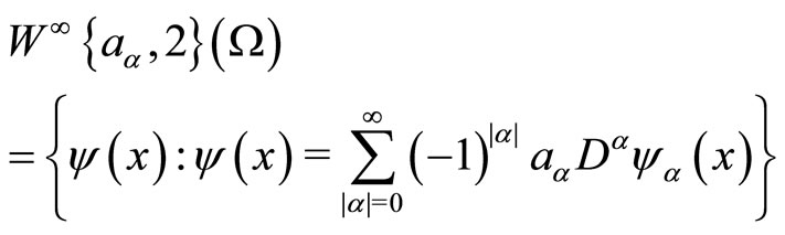
![]() . We define the infinite order Sobolev space
. We define the infinite order Sobolev space  of infinite order of periodic functions
  defined on
  [17-19] as follows:
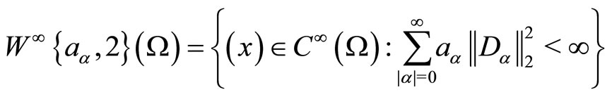
where  is the space of infinite differentiable functions,
  is a numerical sequence and
  is the canonical norm in the space
 , and
, and

 being a multi-index for differentiation,
 .
.
The space  is defined as the formal conjugate space to the space
 , namely:
where  and
and ![]()
The duality pairing of the spaces  and
and  is postulated by the formula

where

From above,  is everywhere dense in
  with topological inclusions and
  denotes the topological dual space with respect to
 , so we have the following chain of inclusions:

We now introduce  which we shall denoted by
 , where
  denotes the space of measurable functions
  such that
endowed with the scalar product
 , L2(Q) is a Hilbert space.
In the same manner we define the spaces
 , and
, and as its formal conjugate.
Also, we have the following chain of inclusions:

The construction of the Cartesian product of n-times to the above Hilbert spaces can be construct, for example

with norm defined by:
where ![]() is a vector function and
is a vector function and
 .
.
Finally, we have the following chain of inclusions:
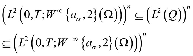
where  are the dual spaces of
 . The spaces considered in this paper are assumed to be real.
3. Mixed Neumann Problem for Infinite Order Hyperbolic System Involving Time Lags
The object of this section is to formulate the following mixed initial boundary value Neumann problem for infinite order hyperbolic system involving time lags which defines the state of the system model.
 (1)
(1)
 (2)
(2)
 (3)
(3)
 (4)
(4)
 (5)
(5)
 (6)
(6)
where  has the same properties as in Section 1. We have

• 
• T is a specified positive number representing a finite time horizon;
• h is a specific positive number representing a time lag;
•  are given real
  functions defined on
 ,
, ![]() respectively;
respectively;
• y is a function defined on Q such that  ;
;
• u, v are functions defined on Q and ![]() such that
such that  and
and ;
;
•  are initial functions defined on
  such that
 .
.
 .
.
The hyperbolic operator  in the state Equation (1) is an infinite order hyperbolic operator and
  [19] is given by:

and

is an infinite order self-adjoint elliptic partial differential operator maps  onto
onto .
.
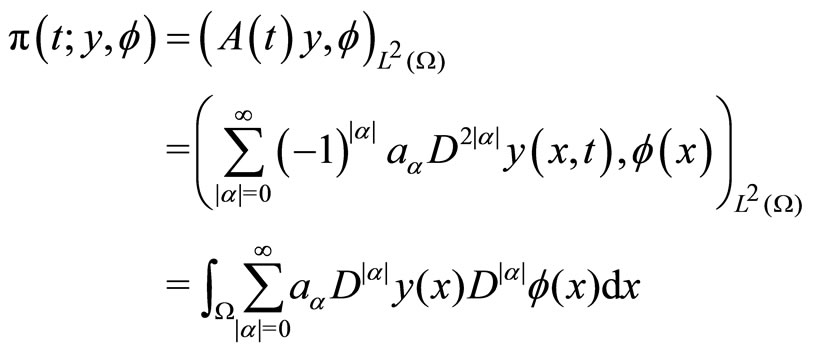
For this operator we define the bilinear form as follows:
Definition 2.1. For each , we define a family of bilinear forms on
  by:
by:
![]()
where  maps
maps  onto
onto  and takes the above form. Then
Lemma 2.1. The bilinear form  is coercive on
  that is
 (7)
(7)
Proof. It is well known that the ellipticity of  is sufficient for the coerciveness of
  on
on  .
.
Then

Also we have:
 (8)
(8)
Equations (1)-(6) constitute a Neumann problem. Then the left-hand side of the boundary condition (5) may be written in the following form:
 (9)
(9)
where  is a normal derivative at
![]() , directed towards the exterior of
, directed towards the exterior of , and
, and  is the
  direction cosine of n, with n being the normal at
 ![]() exterior to
exterior to .
.
Then (5) can be written as:
 (10)
(10)
We shall formulate sufficient conditions for the existence of a unique solution of the mixed boundary value problem (1)-(6) for the case where the boundary control . For this purpose we introduce the Sobolev space
  [20] (p. 6) defined by:
 (11)
(11)
which is a Hilbert space normed by
 (12)
(12)
where the space  denotes the Sobolev space of second order of functions defined on
  and taking values in
  [20] .
The existence of a unique solution for the mixed initial-boundary value problem (1)-(6) on the cylinder Q can be proved using a constructive method, i.e., solving at first Equations (1)-(6) on the sub-cylinder Q1 and in turn on Q2 etc., until the procedure covers the whole cylinder Q. In this way, the solution in the previous step determines the next one.
For simplicity, we introduce the following notation:


Using Theorem 6.1 of [20] (Vol. 2, p. 33), then the following result holds.
Theorem 2.1. Let y0,  ,
,  ,
,  , v and u be given with
 ,
,  ,
,
 ,
,  ,
,  and
and
 and the following compatibility relations:
 (13)
(13)
 (14)
(14)
Then, there exists a unique solution  for the mixed initial-boundary value problem (1)-(6). Moreover,
 , for
, for .
.
4. Problem Formulation and Optimization Theorems
Now, we formulate the optimal control problem for (1)- (6) in the context of the Theorem 2.1, that is .
.
Let us denote by  the space of controls. The time horizon
 ![]() is fixed in our problem.
is fixed in our problem.
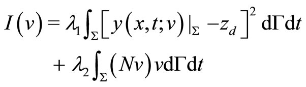
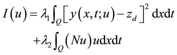
The performance functional is given by:
 (15)
(15)
where , and
, and 
 is a given element in
 ; N is a positive linear operator on
  into
into .
.
Control constraints: We define the set of admissible controls  such that
 (16)
(16)
Let  denote the solution of the mixed initialboundary value problem (1)-(6) at
  corresponding to a given control
 . We note from Theorem 2.1 that for any
  the performance functional (15) is well-defined since
 .
.
Making use of the Loins’s scheme we shall derive the necessary and sufficient conditions of optimality for the optimization problem (1)-(6), (15), (16). The solving of the formulated optimal control problem is equivalent to seeking a  such that
From the Lion’s scheme [21] (Theorem 1.3 of, p. 10), it follows that for  a unique optimal control
  exists. Moreover,
  is characterized by the following condition:
 (17)
(17)
For the performance functional of form (15) the relation (17) can be expressed as
 (18)
(18)
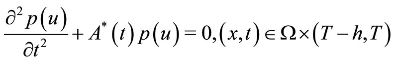
In order to simplify (18), we introduce the adjoint equation, and for every , we define the adjoint variable
  as the solution of the equations:
 (19)
(19)
 (20)
(20)
 (21)
(21)
 (22)
(22)
 (23)
(23)
 (24)
(24)
where 
 (25)
(25)
As in the above section with change of variables, i.e. with reversed sense of time. i.e.,  , for given
  and any
 , there exists a unique solution
  for problem (19)-(24).
The existence of a unique solution for the problem (19)-(24) on the cylinder Q can be proved using a constructive method. It is easy to notice that for given  and v, the problem (19)-(24) can be solved backwards in time starting from
 , i.e. first solving (19)-(24) on the sub-cylinder
  and in turn on
 , etc. until the procedure covers the whole cylinder Q. For this purpose, we may apply Theorem 2.1 (with an obvious change of variables). Hence, using Theorem 2.1, the following result can be proved.
Lemma 3.1. Let the hypothesis of Theorem 2.1 be satisfied. Then for given  and any
 , there exists a unique solution
  for the adjoint problem (19)-(24).
We simplify (18) using the adjoint equation (19)-(24). For this purpose denoting by  and
and  respectively, setting
  in (19)- (24), multiplying both sides of (19), (20) by y(v) – y(v*), then integrating over
  and
and  respectively and then adding both sides of (19), (20), we get
 (26)
(26)
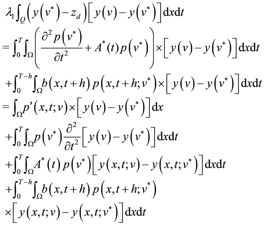
Using the Equation (1), the second integral on the right-hand side of (26) can be written as
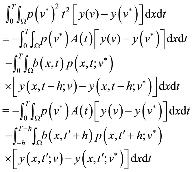 (27)
(27)
Using Green’s formula, the third integral on the righthand side of (26) can be written as
 (28)
(28)
Using the boundary condition (5), one can transform the second integral on the right-hand side of (28) into the form:
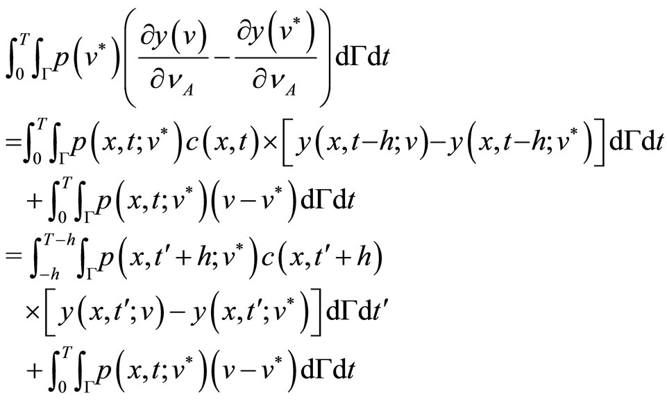 (29)
(29)
The last component in (28) can be rewritten as
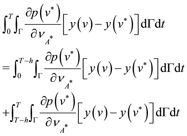 (30)
(30)
Substituting (29) and (30) into (28), and then (27), (28) into (26), we obtain
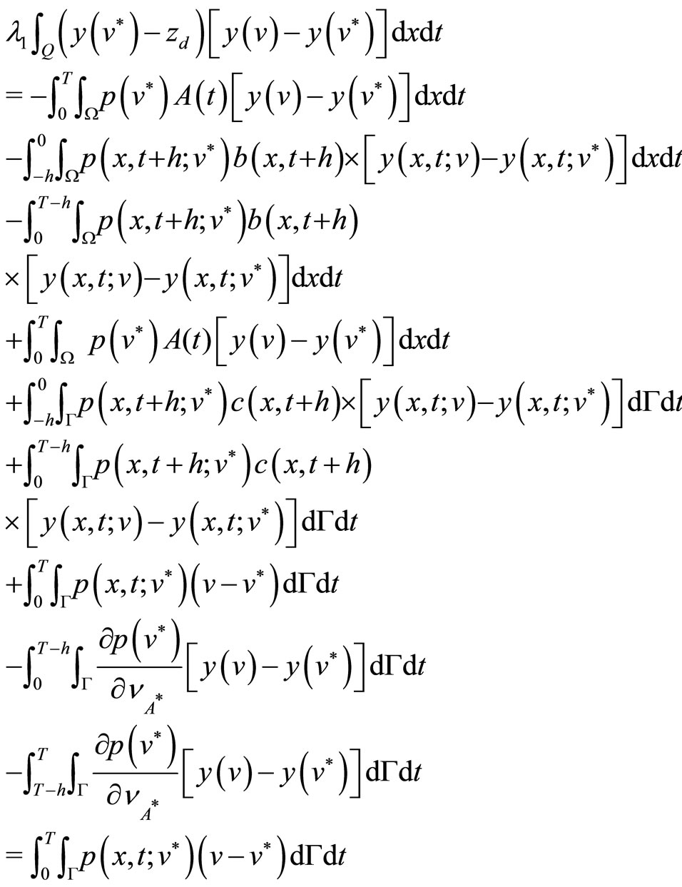 (31)
(31)
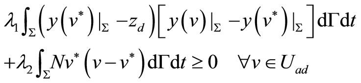
Substituting (31) into (18) gives
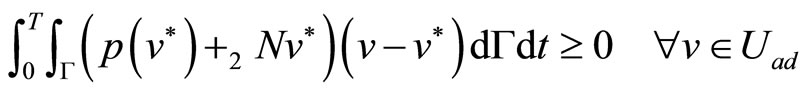 (32)
(32)
The foregoing result is now summarized.
Theorem 3.1. For the problem (1)-(6), with the performance functional (15) with  and
and  and with conditions (16), there exists a unique optimal control
  which satisfies the maximum condition (32).
Mathematical Examples
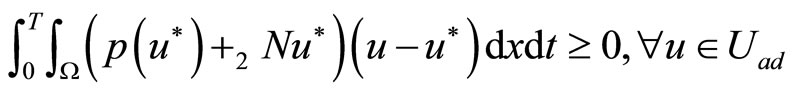
Example 3.1. Consider now the particular case where  (no constraints case). Thus the maximum condition (32) is satisfied when

If N is the identity operator on , then from the Lemma 3.1 follows that
 .
.
Example 3.2. We can also consider an analogous optimal control problem where the performance functional is given by:
 (33)
(33)
where .
.
From Theorem 2.1 and the Trace Theorem [20] (Vol. 2, p. 9), for each , there exists a unique solution
  with
with . Thus,
  is well defined. Then, the optimal control
  is characterized by:
 (34)
(34)
We define the adjoint variable  as the solution of the equations:
 (35)
(35)
 (36)
(36)
 (37)
(37)
 (38)
(38)
 (39)
(39)
 (40)
(40)
As in the above section, we have the following result.
Lemma 3.2. Let the hypothesis of Theorem 2.1 be satisfied. Then, for given  and any
  , there exists a unique solution
 to the adjoint problem (35)-(40).
Using the adjoint Equations (35)-(40) in this case, the condition (34) can also be written in the following form
 (41)
(41)
The following result is now summarized.
Theorem 3.2. For the problem (1)-(6) with the performance function (33) with  and
and , and with constraint (16), and with adjoint Equations (35)-(40), there exists a unique optimal control
  which satisfies the maximum condition (41).
Example 3.3. Case: . We can also consider an analogous optimal control problem where the performance functional is given by:
 (42)
(42)
where .
.
From Theorem 2.1 and the Trace Theorem [20] (Vol. 2, p. 9), for each , there exists a unique solution
 . Thus, I is well defined. Then, the optimal control
  is characterized by
 (43)
(43)
We define the adjoint variable  as the solution of the equations:
 (44)
(44)
 (45)
(45)
 (46)
(46)
 (47)
(47)
 (48)
(48)
 (49)
(49)
As in the above section, we have the following result.
Lemma 3.3. Let the hypothesis of Theorem 2.1 be satisfied. Then, for given  and any
 , there exists a unique solution
  to the adjoint problem (44)-(49).
Using the adjoint equations (44)-(49) in this case, the condition (43) can also be written in the following form:
 (50)
(50)
The following result is now summarized.
Theorem 3.3. For the problem (1)-(6), (44)-(49), (16) with ,
,  , there exists a unique optimal control
  which satisfies the maximum condition (50).
5. Generalization
The optimal control problems presented her can be extended to certain different two cases. Case 1: Optimal control for  coupled infinite order hyperbolic systems involving constant time lags. Case 2: Optimal control for
 ![]() coupled infinite order hyperbolic systems involving constant time lags. Such extension can be applied to solving many control problems in mechanical engineering.
coupled infinite order hyperbolic systems involving constant time lags. Such extension can be applied to solving many control problems in mechanical engineering.
Case 1: Optimal control for 2 × 2 coupled infinite order hyperbolic systems involving constant time lags.
We will extend the discussions to study the optimal control for  coupled infinite order hyperbolic systems involving constant time lags. We consider the case where
 , the performance functional is given by:
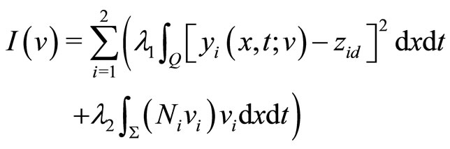 (51)
(51)
where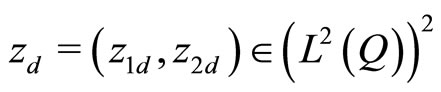 .
.
The following results can now be proved.
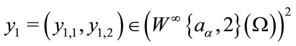
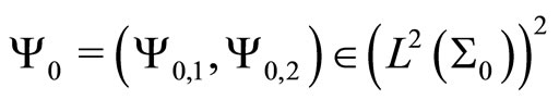
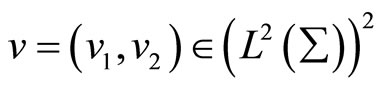
Theorem 4.1. Let ,
,  ,
,  ,
,  ,
, ![]() and
and ![]() be given with
be given with
 ,
,
 ,
,
 ,
,
 ,
,
and .
.
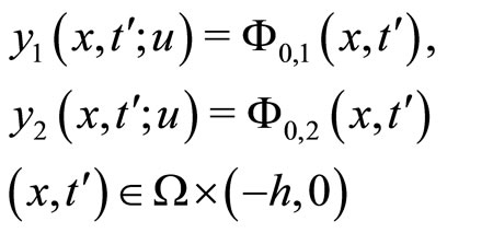
Then, there exists a unique solution
 for the following mixed initial-boundary value problem:
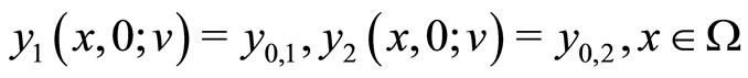
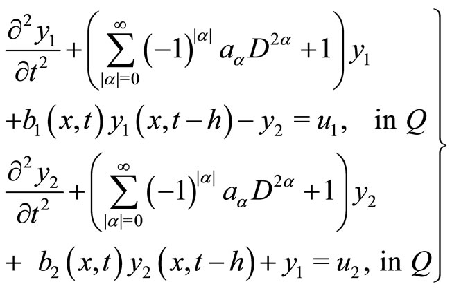 (52)
(52)
 (53)
(53)
 (54)
(54)
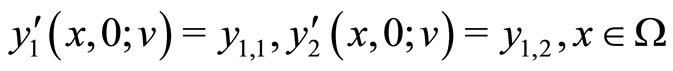 (55)
(55)
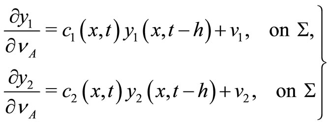 (56)
(56)
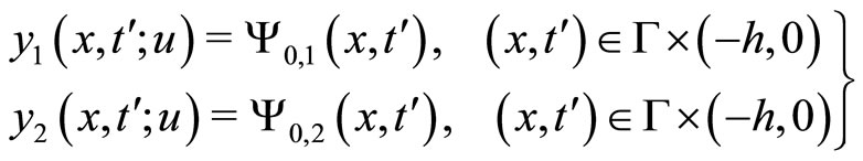 (57)
(57)
where

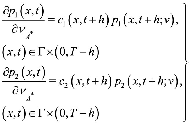
Lemma 4.1. Let the hypothesis of Theorem 4.1 be satisfied. Then for given  and any
 , there exists a unique solution
  for the adjoint problem:
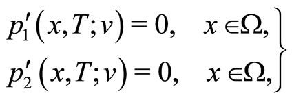
 (58)
(58)
 (59)
(59)
 (60)
(60)
 (61)
(61)
 (62)
(62)
 (63)
(63)
Theorem 4.2. The optimal control
 is characterized by the following maximum condition
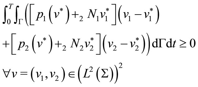 (64)
(64)
where  is the adjoint state.
The foregoing result is now summarized.
Theorem 4.3. For the problem (52)-(57) with the performance function (51) with
 and
and , and with constraint:
  is closed, convex subset of
 , and with adjoint equations (58)-(63), then there exists a unique optimal control
which satisfies the maximum condition (64).
Case 2: Optimal control for n × n coupled infinite order hyperbolic systems involving constant time lags.
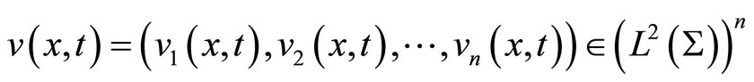
We will extend the discussion to n × n coupled infinite order hyperbolic systems involving constant time lags. We consider the case where
 , the performance functional is given by (El-Saify, 2005; 2006):
 (65)
(65)
where .
.
The following results can now be proved.
Theorem 4.4. Let ,
,  ,
,  ,
,  ,
, ![]() and
and ![]() be given with
be given with
 ,
,
 ,
,
 ,
,
 ,
,

and .
.
Then, there exists a unique solution
 for the following mixed initial-boundary value problem:
  we have
 (66)
(66)
 (67)
(67)
 (68)
(68)
 (69)
(69)
 (70)
(70)
 (71)
(71)
where


 are given real
  functions defined on
 , respectively, h is a time lags,
 are initial functions defined on
  respectively.
The operator  is an
is an ![]() matrix takes the form [22-25] (El-Saify & Bahaa 2000; 2001; 2002; 2003).
matrix takes the form [22-25] (El-Saify & Bahaa 2000; 2001; 2002; 2003).
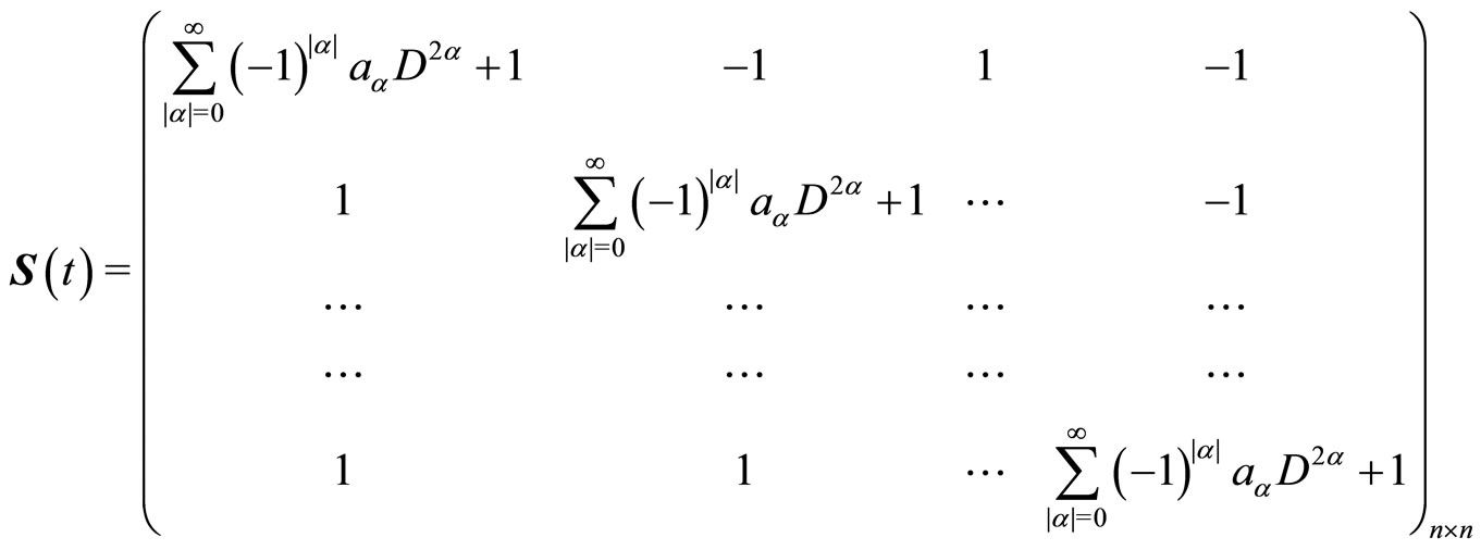
That is
 (72)
(72)
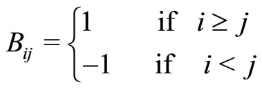
where
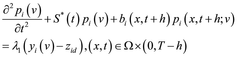
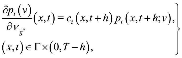
Lemma 4.2. Let the hypothesis of Theorem 4.4 be satisfied. Then for given
 and any
 , there exists a unique solution

for the adjoint problem: , we have
 (73)
(73)
 (74)
(74)
 (75)
(75)
 (76)
(76)
 (77)
(77)
 (78)
(78)
Theorem 4.5. The optimal control
is characterized by the following maximum condition
 (79)
(79)
where
is the adjoint state.
The foregoing result is now summarized.
Theorem 4.6. For the problem (66)-(71) with the performance function (65) with
 and
and , and with constraint:
  is closed, convex subset of
 , and with adjoint Equations (73)-(78), then there exists a unique optimal control

which satisfies the maximum condition (79).
In the case of performance functionals (15, 33, 42, 51 and 65) with  and
and , the optimal control problem reduces to minimization of the functional on a closed and convex subset in a Hilbert space. Then, the optimization problem is equivalent to a quadratic programming one, which can be solved by the use of the well-known Gilbert algorithm.
6. Conclusions
The optimization problem presented in the paper constitutes a generalization of the optimal boundary control problem of a second order hyperbolic systems involving constant time lags appearing in the boundary condition have been considered in [4-16,22].
In this paper, we have considered the boundary control problem for infinite order hyperbolic system and also for  infinite order hyperbolic systems involving constat time lags appearing both in the state equations and in the Neumann boundary conditions. We can also consider the boundary optimal control problem for
  infinite order parabolic or hyperbolic systems with timevarying delays appearing in the state equations and in the Neumann or Dirichlet boundary conditions. We can also consider the boundary optimal control problem for
  infinite order hyperbolic systems with timevarying delays appearing in the integral form with
  or
or  both in the state equations and in the Neumann or Dirichlet boundary conditions.
Also it is evident that by modifying:
• The boundary conditions, (Dirichlet, Neumann, mixed, etc.);
• The nature of the control (distributed, boundary, etc.);
• The nature of the observation (distributed, boundary, etc.);
• The initial differential system;
• The time delays (constant time delays, time-varying delays, multiple time-varying delays, time delays given in the integral form, etc.);
• The number of variables (finite number of variables, infinite number of variables systems, etc.);
• The type of equation (elliptic, parabolic, hyperbolic, etc.);
• The order of equation (second order, Schrödinger, infinite order, etc.);
• The type of control (optimal control problem, timeoptimal control problem, etc.), an infinity of variations on the above problem are possible to study with the help of [21] and Dubovitskii-Milyutin formalisms [23-32]. Those problems need further investigations and form tasks for future research. These ideas mentioned above will be developed in forthcoming papers.
REFERENCES
- P. K. C. Wang, “Optimal Control of Parabolic Systems with Boundary Conditions Involving Time Delays,” SIAM Journal on Control, Vol. 13, No. 2, 1975, pp. 274-293. doi:10.1137/0313016
- G. Knowles, “Time-Optimal Control of Parabolic Systems with Boundary Conditions Involving Time Delays,” Journal of Optimization Theory and Applications, Vol. 25, No. 4, 1978, pp. 563-574. doi:10.1007/BF00933521
- K. H. Wong, “Optimal Control Computation for Parabolic Systems with Boundary Conditions Involving Time Delays,” Journal of Optimization Theory and Applications, Vol. 53, No. 3, 1987, pp. 475-507. doi:10.1007/BF00938951
- A. Kowalewski, “Optimal Control of Hyperbolic System with Boundary Condition Involving a Time-Varying Lag,” Proceedings of the IMACS/IFAC International Symposium on Modeling and Simulation of DPS, Hiroshima, 6-9 October 1987, pp. 462-467.
- A. Kowalewski, “Boundary Control of Hyperbolic Systems with Boundary Condition Involving a Time Delay,” Analysis and Optimization of Systems, Vol. 111, 1988, pp. 507-518. doi:10.1007/BFb0042240
- A. Kowalewski, “Optimal Control of Distributed Hyperbolic System with Boundary Condition Involving a Time Lag,” Automatic Remote Control, XXXIII, 1988, pp. 537- 545.
- A. Kowalewski, “Optimal Control of Distributed Parabolic System Involving Time Lags,” IMA Journal of Mathematical Control and Information, Vol. 7, No. 4, 1990, pp. 375-393. doi:10.1093/imamci/7.4.375
- A. Kowalewski, “Optimal Control of Parabolic Systems with Time-Varying Lags,” IMA Journal of Mathematical Control and Information, Vol. 10, No. 2, 1993, pp. 113- 129. doi:10.1093/imamci/10.2.113
- A. Kowalewski, “Optimal Control of a Distributed Parabolic Systems with Multiple Time-Varying Lags,” International Journal of Control, Vol. 69, No. 3, 1998, pp. 361-381. doi:10.1080/002071798222712
- A. Kowalewski, “Optimization of Parabolic Systems with Deviating Arguments,” International Journal of Control, Vol. 72, No. 11, 1999, pp. 947-959. doi:10.1080/002071799220498
- A. Kowalewski and J. Duda, “On Some Optimal Control Problem for a Parabolic System with Boundary Condition Involving a Time-Varying Lag,” IMA Journal of Mathematical Control and Information, Vol. 9, No. 2, 1992, pp. 131-146. doi:10.1093/imamci/9.2.131
- A. Kowalewski and J. Duda, “An Optimization Problem Time Lag Distributed Parabolic Systems,” IMA Journal of Mathematical Control and Information, Vol. 21, No. 1, 2004, pp. 15-31. doi:10.1093/imamci/21.1.15
- W. Kotarski, H. A. El-Saify and G. M. Bahaa, “Optimal Control of Parabolic Equation with an Infinite Number of Variables for Non-Standard Functional and Time Delay,” IMA Journal of Mathematical Control and Information, Vol. 19, No. 4, 2002, pp. 461-476. doi:10.1093/imamci/19.4.461
- W. Kotarski and G. M. Bahaa, “Optimality Conditions for Infinite Order Hyperbolic Problem with Non-Standard Functional and Time Delay,” Journal of Information & Optimization Sciences, Vol. 28, No. 6, 2007, pp. 315-334.
- H. A. El-Saify, “Optimal Control for n × n Parabolic System Involving Time Lag,” IMA Journal of Mathematical Control and Information, Vol. 22, No. 3, 2005, pp. 240-250. doi:10.1093/imamci/dni011
- H. A. El-Saify, “Optimal Boundary Control Problem for n × n Infinite Order Parabolic Lag System,” IMA Journal of Mathematical Control and Information, Vol. 23, No. 4, 2006, pp. 433-445. doi:10.1093/imamci/dni065
- J. A. Dubinskii, “Sobolev Spaces of Infinite Order and the Behavior of Solution of Some Boundary Value Problems with Unbounded Increase of the Order of the Equation,” Mathematics of the USSR-Sbornik, Vol. 27, No. 2, 1975, p. 143. doi:10.1070/SM1975v027n02ABEH002506
- J. A. Dubinskii, “Non-Triviality of Sobolev Spaces of Infinite Order for a Full Euclidean Space and a Torus,” Mathematics of the USSR-Sbornik, Vol. 100, 1976, pp. 436-446.
- J. A. Dubinskii, “Sobolev Spaces of Infinite Order and Differential Equations,” Springer-Verlag, New York, 1986.
- J. L. Lions and E. Magenes, “Non-Homogeneous Boundary Value Problem and Applications,” Springer-Verlag, New York, 1972.
- J. L. Lions, “Optimal Control of Systems Governed by Partial Differential Equations,” Springer-Verlag, New York, 1971.
- H. A. El-Saify and G. M. Bahaa, “Optimal Control for n × n Hyperbolic Systems Involving Operators of Infinite Order,” Mathematica Slovaca, Vol. 52, No. 4, 2002, pp. 409-424.
- G. M. Bahaa, “Quadratic Pareto Optimal Control of Parabolic Equation with State-Control Constraints and Infinite Number of Variables,” IMA Journal of Mathematical Control and Information, Vol. 20, No. 2, 2003, pp. 167-178. doi:10.1093/imamci/20.2.167
- G. M. Bahaa, “Time-Optimal Control Problem for Infinite Order Parabolic Equation with Control Constraints,” Differential Equations and Control Processes. The Electronic Journal, Vol. 4, 2005, pp. 64-81. http://www.neva.ru/journal
- G. M. Bahaa, “Optimal Control for Cooperative Parabolic Systems Governed by Schrödinger Operator with Control Constraints,” IMA Journal of Mathematical Control and Information, Vol. 24, No. 1, 2007, pp. 1-12. doi:10.1093/imamci/dnl001
- G. M. Bahaa, “Quadratic Pareto Optimal Control for Boundary Infinite Order Parabolic Equation with StateControl Constraints,” AMO-Advanced Modeling and Optimization, Vol. 9, 2007, pp. 37-51.
- G. M. Bahaa, “Optimal Control Problems of Parabolic Equations with an Infinite Number of Variables and with Equality Constraints,” IMA Journal of Mathematical Control and Information, Vol. 25, No. 1, 2008, pp. 37-48. doi:10.1093/imamci/dnm002
- G. M. Bahaa and W. Kotarski, “Optimality Conditions for n × n Infinite Order Parabolic Coupled Systems with Control Constraints and General Performance Index,” IMA Journal of Mathematical Control and Information, Vol. 25, No. 1, 2008, pp. 49-57. doi:10.1093/imamci/dnm003
- W. Kotarski and G. M. Bahaa, “Optimal Control Problem for Infinite Order Hyperbolic System with Mixed Control-State Constraints,” European Journal of Control, Vol. 11, No. 2, 2005, pp. 150-156. doi:10.3166/ejc.11.150-156
- W. Kotarski, H. A. El-Saify and G. M. Bahaa, “Optimal Control Problem for a Hyperbolic System with Mixed Control-State Constraints Involving Operator of Infinite Order,” International Journal of Pure and Applied Mathematics, Vol. 1, No. 3, 2002, pp. 239-252.
- A. Kowalewski, “Time-Optimal Control of Infinite Order Hyperbolic Systems with Time Delays,” International Journal of Applied Mathematics and Computer Science, Vol. 19, No. 4, 2009, pp. 597-608. doi:10.2478/v10006-009-0047-x
- A. Kowalewski and A. Krakowiak, “Time-Optimal Boundary Control of Infinite Order Parabolic System with Time Lags,” International Journal of Applied Mathematics and Computer Science, Vol. 18, No. 2, 2008, pp. 189-198. doi:10.2478/v10006-008-0017-8