Journal of Modern Physics
Vol.4 No.5(2013), Article ID:31414,7 pages DOI:10.4236/jmp.2013.45080
Localisation Inverse Problem of Absorbing Laplacian Transport
École Centrale Paris, Laboratoire de MSS-MAT, Grande Voie des Vignes, Châtenay-Malabry Cedex, France
Email: ibrahim.baydoun@ecp.fr
Copyright © 2013 Ibrahim Baydoun. This is an open access article distributed under the Creative Commons Attribution License, which permits unrestricted use, distribution, and reproduction in any medium, provided the original work is properly cited.
Received December 24, 2012; revised February 6, 2013; accepted March 7, 2013
Keywords: Laplacian Transport; Dirichlet-to-Neumann Operators; Inverse Problem; Conformal Mapping
ABSTRACT
We study the localisation inverse problem corresponding to Laplacian transport of absorbing cell. Our main goal is to find sufficient Dirichelet-to-Neumann conditions insuring that this inverse problem is uniquely soluble. In this paper, we show that the conformal mapping technique is adopted to this type of problem in the two dimensional case.
1. Introduction
The theory of Dirichlet-to-Neumann operators is the basis of many research domains in analysis, particularly, those concerning Laplacian transports. It is also very important in mathematical-physics, geophysics, electrochemistry. Moreover, it is very useful in medical diagnosis, such as electrical impedance tomography, as showing in the following example:
Example 1. In 1989, J. Lee and G. Uhlmann have introduced an example on the determination of conductivity matrix field , for
, for  in a bounded open domain
 , see e.g. [1]. This example is related to measuring of elliptic Dirichlet-to-Neumann map for associated conductivity equation, see e.g. [1]. Notice that the solution of this problem has a lot of practical applications in various domains overall in medicine, which is an important diagnostic tool, e.g. in the electrical impedance tomography; the tissue in the human body is an example of highly anisotropic conductor [2].
Under assumption that there are no sources or sinks of current the potential  for a given voltage
  on the (smooth) boundary
  of
of  is a solution of the Dirichlet problem:
(P1) 
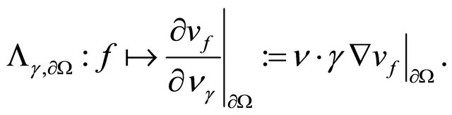
Then the corresponding to (P1) Dirichlet-to-Neumann map (operator)  is (formally) defined by [3] as follows:
 (1.1)
(1.1)
Here  is the unit outer-normal vector to the boundary at
  and the function
  is a solution of the Dirichlet problem (P1).
Dirichlet-to-Neumann operator (1.1) is also called the voltage-to-current map, since the function  gives the induced current flux trough the boundary
 . The key (inverse) problem is whether on can determine the conductivity matrix
  by knowing electrical boundary measurements, i.e. the corresponding Dirichlet-to-Neumann operator? In general this operator does not determine the matrix
  uniquely, see e.g. [4].
The main question in this context is to find sufficient conditions insuring that the inverse problem is uniquely soluble.
The problem of electrical current flux in the form (P1) is an example of so-called diffusive Laplacian transport. Besides the voltage-to-current problem, the motivation to study this kind of transport comes for instance, from the transfer across biological membranes, see e.g. [5,6]:
Example 2. Let some species of concentration  , diffuse stationary in the isotropic bulk
  from a (distant) source localised on the closed boundary
  towards a semipermeable compact interface
  of cell
 , where they disappear at a given rate
 . Then the steady field of concentrations (Laplacian transport with a diffusion coefficient
 ) obeys the set of equations:
(P2) 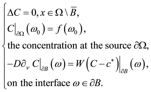
Here  is the constant concentration of the species inside cell
 .
.
Now, similar to (1.1), we can associate with the problem (P2) a Dirihlet-to-Neumann operator
 (1.2)
(1.2)
with domain  belongs to a certain Sobolev space, see Section 2.
The advantage of this approach is that as soon as the operator (1.2) is defined, one can apply it to study the mixed boundary value problem (P2). This gives, in particularly, the value of the particle flux due to Laplacian transport across the membrane . Moreover, the total current across the boundary
  can be defined (for given f) in term of Dirihlet-to-Neumann operator (1.2) as follows:
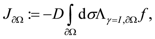 (1.3)
(1.3)
where  designed the differential element relative to
 .
.
The aim of the present paper is to show how can apply the theory of Dirichlet-to-Neumann operators on the localisation inverse problem in the framework of application outlined in problem (P2), which consists in finding the sufficient (Dirihlet-to-Neumann) conditions to localise the position of cell  from the experimentally measurable macroscopic response parameters.
In Section 2, we introduce the existence and uniqueness for the solution of problem (P2). In Section 3, we present our main results which consist in showing that total current (1.3), involving Dirihlet-to-Neumann operator (1.2), can resolve the localisation inverse problem in the two-dimensional case, when the compact . We allow an explicit calculations for the solution of problem (P2) from Dirichlet-Neumann boundary conditions. Whereas for this solution, we use a method of conformal mapping for harmonic functions in doubly connected domains
 .
.
2. Uniqueness of the Problem (P2)
We suppose that  and
and  be open bounded domains in
  with
with  -smooth disjoint boundaries
  and
and , that is
  and
and  .
.
Then the unit outer-normal to the boundary  vector-field
  is well-defined, and we consider the normal derivative in (P2) as the interior limit:
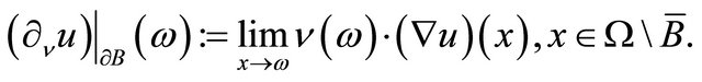 (2.1)
(2.1)
The existence of the limit (2.1) as well as the restriction  is insured since
  has to be harmonic solution of problem (P2) for
  -smooth boundaries
  [7].
[7].
Now, we introduce some indispensable standard notations and definitions, see [8]. Let  be Hilbert space
  on domain
  and
and  denote the corresponding boundary space. We denote by
  the Sobolev space of
  -functions, whose
  -derivatives are also in
 , and similar,
  is the Sobolev space of
  -functions on the
  -smooth boundary
 .
.
Proposition 2.1 Let  for
for  -smooth boundaries
 . Then the Dirichlet-Neumann problem (P2) has a unique (harmonic) solution in domain
 .
.
Proof. For existence we refer to [7]. To prove the uniqueness, we consider the problem (P2) for  and
and . Then by Gauss-Ostrogradsky theorem, one gets that the corresponding solution
  yields:
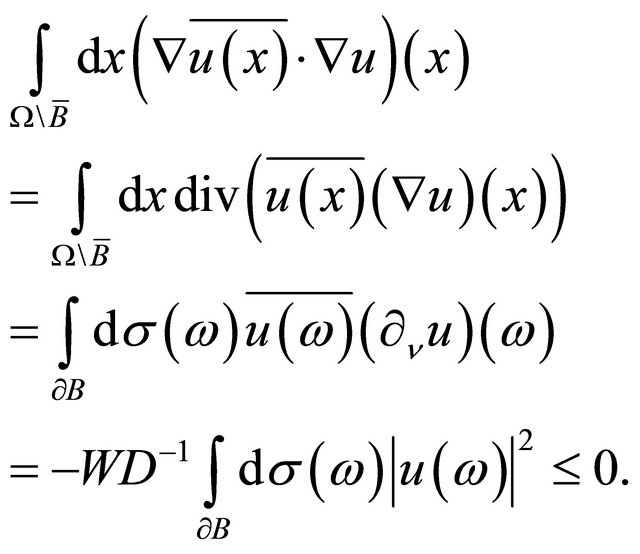 (2.2)
(2.2)
The estimate (2.2) implies that . Hence by the boundary condition one gets
 , and from
 we obtain that for
 , the harmonic function
  for
for . □
. □
The next statement is a key for analysis of inverse localisation problems:
Proposition 2.2 Consider two problems (P2) corresponding to a bounded domain  with C2-smooth boundary
  and to two subsets
  and
and  with the same smoothness of the boundaries
 . If for solutions
  of these problems one has
 (2.3)
(2.3)
then .
.
Proof. By virtue of  and by condition (2.3), the problem (P2) has two solutions for identical external (on
 ) and internal (on
  and
and ) Robin boundary conditions. Then by the standard arguments based on the Holmgren uniqueness theorem [9] for harmonic functions on
 , one obtains that
  . □
. □
3. Inverse Problem: Conformal Mapping
Let  and
and  be respectively open bounded domains in
  with
with  -smooth disjoint boundaries
 and
and , where
and  are two circles respectively with radius
  and
and .
.
In the sequel, we denote by  the distance between the two centers
 .
.
The solution of the inverse localisation problem is decomposed into two steps:
In the first step, we introduce the necessary conformal mapping, see [10]. There are two reasons that make interest for using this technique, indeed the convenable conformal mapping :
:
(a) Transforms two non-concentric circles into two concentric circles.
(b) For any harmonic function ,
,  still harmonic, see Proposition 3.1.
With this technique, we transform problem (P2) to another problem (P2)*, whose (P2)* has as solution an harmonic function also, and as domains  and
and  which are concentric.
Therefore, we can find easily the general form for the solution of (P2)*, and consequently, we conclude the necessary coefficients for the general solution of problem (P2), with which we will be able to resolve its inverse problem.
In the next step, we are interested by resolving the localisation inverse problem using the explicit formula of , which will be calculated in terms of (measurable) Dirichlet-Neumann boundary hypothesis on
 .
.
Proposition 3.1 Let  be a conformal mapping defined by:

If  is an harmonic function in
 , then the composition

is an harmonic function in .
.
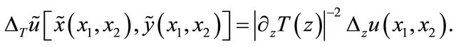
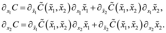
In particular, by distinguishing explicitly the Laplacian in different coordinates,  and
and
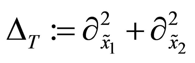 , one obtains:
3.1. Necessary Conformal Mapping
Let  be the conformal mapping defined by:1
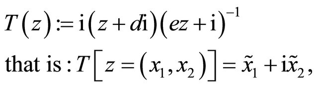 (3.1)
(3.1)
where:
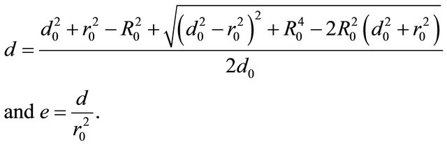
(3.2)
Remark 1 We define the conformal mapping  relatively to the orthonormal reference with origin
  and axis
  which is keen on the line
  in the sense of the vector
 .
.
Corollary 3.2 T transforms  and
and
 from non-concentric circles to concentric circles
  and
and , where
  is defined by:
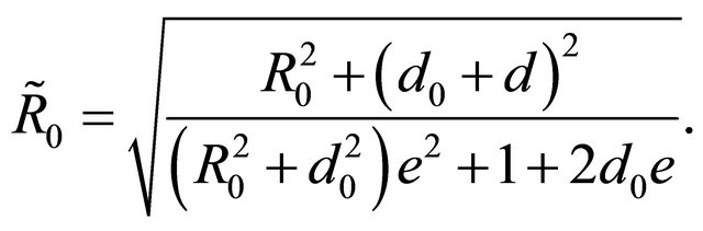 (3.3)
(3.3)
Remark 2 Notice that when , the mapping
  converges to the identity function.
3.2. Problem (P2)*
Let  and
and  be respectively the values of the normal derivative
  and
and  with the new variables
 , i.e:
Then, if we make the substitution , then by using the conformal mapping given in (3.1), we show from proposition 3.1 that the problem (P2) can be transformed to problem (P2)*, which obeys the set of equations:
(P2)* 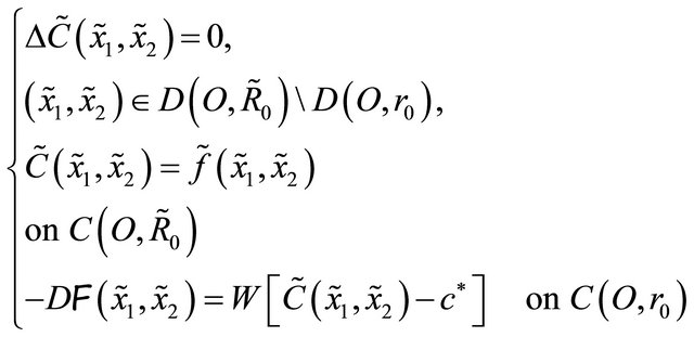
In the sequel, we denote by  and
and  the polar coordinates associated to the variables
 .
.
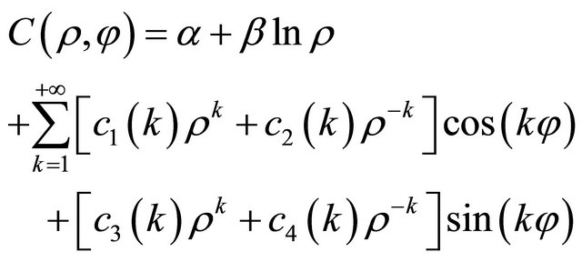
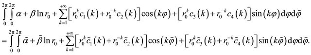
Corollary 3.3 The solution of the problem (P2)* gets the form:
 (3.4)
(3.4)
Proof. As  is harmonic, then the proof follows, see [10]. □
Hereinafter, we need to make explicit  in order to calculate the coefficients of the development (3.4).
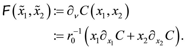
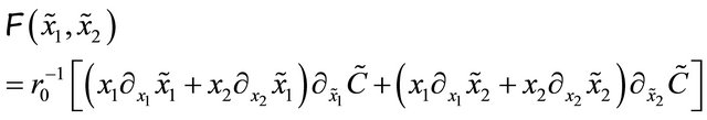
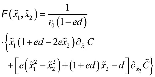
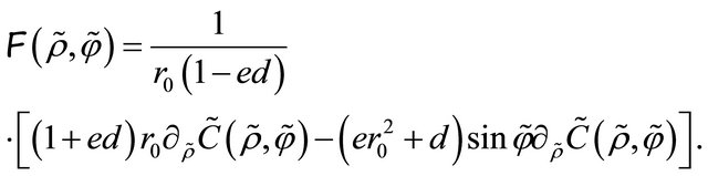
Proposition 3.4 The function  is given by:
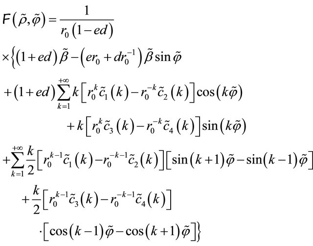
(3.5)
Proof. Since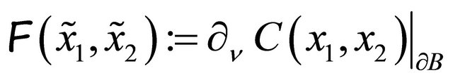 , we deduce from the definition of
  that:
that:
 (3.6)
(3.6)
We need firstly to calculate  and
and  in terms of
 . By virtue of the substitution
 , we obtain the following differential relation:
Then by comparison, we conclude that:
 (3.7)
(3.7)
Substitute Equation (3.7) in Equation (3.6), one obtains:
(3.8)
Recall that Equation (3.1) gives us a relation between the variables  and
and . Then, the quantities
 and
and  in Equation
(3.8) can be calculated in terms of . Therefore we have:
Finally, if we replace  and
and  by their associated polar coordinates
 , then we can rewrite
  in terms of
  and
and  (due to the relation between polar derivatives and cartesian derivatives) as follows:
 (3.9)
(3.9)
Therefore, it is enough to replace  by its value given in Equation (3.4). □
In order to resolve problem (P2)*, we need to make explicit . So, the change of variables given in Equation (3.1), allows us to express
  with the following Fourier series:
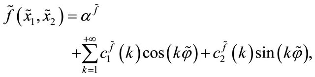 (3.10)
where:
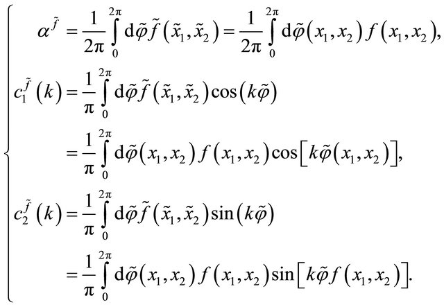
Remark 3 Notice that the coefficients of (16) depend only of:
1.  given from the change of variables due to (3.1).
2. f which is the external condition boundary of problem (P2).
Proposition 3.5 The coefficients of Equation (3.4) are given by:
 (3.11)
Proof. First boundary condition of problem (P2)* implies: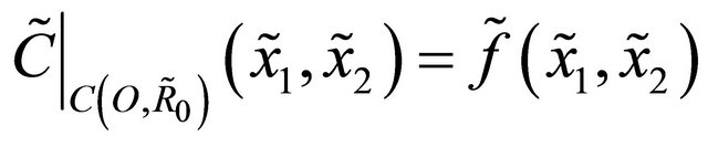 . Then, by replacing
 and
and  by their values given respectively in (3.4) and (3.10), we obtain after identification that:

Afterwards, from the second boundary condition in problem (P2)*, we have
 . Then, by the similar manner, we deduce from (3.5) and (3.4) that:
Finally, one has a system of six equations with six unknowns and
and . The solution of this system ends the proof. □
Remark 4 Notice that the proof of Proposition 3.5 show us the advantage of conformal mapping technique. Indeed, the identification between Fourier series on the boundary conditions of problem (P2)* is easily calculated because its boundaries are two concentric circles, and consequently its radius are constant. But, it is not the case in problem (P2), because here its boundaries are non-concentric, whose its radius depend of polar angle.
Remark 5 For the inverse problem, we will just need the explicit value of  and
and , that why we didn’t make explicit the other coefficients values for the Fourier series of
 .
.
3.3. Localisation Inverse Problem
For resolving the inverse problem, we need the following:
(i) First, we aim to calculate the total flux  across the external boundary
 . For that, we need to express the solution
  of problem (P2) in terms of Fourier series.
(ii) Second, we aim to find an equation for .
.
In the sequel, we denote by  and
and  the polar coordinates associated to the initial variables
 .
.
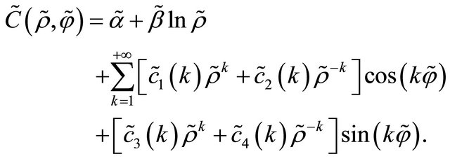
(i) The solution of problem (P2) gets the following form:
 (3.12)
where  and
and  for all
  , are the Fourier coefficients of
 .
.
Corollary 3.6 The total flux  and
and  satisfy the following:
 (3.13)
Proof. Since the differential element  at boundary
  are respectively equal to
 , then by inserting (3.12) in (1.2), we deduce that:
where  and
and  designed respectively local current and outer-normal vector at arbitrary point
 .
.
On the other hand, by Gauss-Ostrogradsky theorem, one gets:
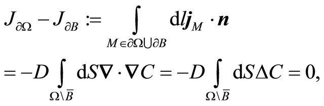
where  is the areal differential element. Therefore, (19) is deduced. □
(ii) We now state the following corollary and proposition which will be important to find a relation between the coefficients  and
and  involving
 .
.
Corollary 3.7
 (3.14)
Proof. Substitute  in the second boundary condition of problem (P2) (at the interface
  of cell
 ) by its value given in Equation (3.12), therefore the proof follows by identification (between two Fourier series). □
Proposition 3.8
 (3.15)
Proof. Since , one gets also
 . But, we have
 , then
 .
.
On the other hand,  varies in
 . So, by applying the double integral on the domain
 for the equality
 , and by replacing
  and
and  by their values given respectively in Equations (3.4) and (3.12), we deduce that:
Then Equation (3.15) follows from Fubini’s theorem. □
Finally, we aim to find the equation satisfied by .
.
In fact, by inserting (3.13) and (3.14) in Equation (3.15), we obtain:
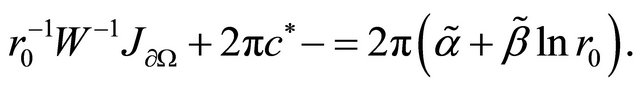 (3.16)
4. Conclusions
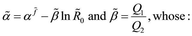
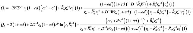
From Proposition 3.5, we remark that  and
and  are calculated in terms of
  and
and , which their formulae given in (3.2) and (3.3) depend of
  and the coefficients of (3.10).
Then, Equation (3.16) becomes an equation of the only unknown  involving the parameters
  (1.3) and
  (see Remark 3), which are the Dirichlet-toNeumann hypothesis of problem (P2) on the external boundary, and we can found them from an experimental measures.
To summarize, we have found an equation for , which is the distance between the center
  of cell
  and the center
  of
of , so it remains to find the position of the center
 . In fact:
Let  and
and  be two points at the external boundary
  whose the norm of the local current
  reaches respectively its maximum and minimum values, see Figure 1. Then, from the symmetry of the shape, we deduce that the center
  of cell
  is localized at the line passed by the points
 ,
,  and
and , exactly between
  and
and  where the distance
  between
  and
and  is given by Equation (3.16).
By conclusion, we can now answer the question posed in the introduction about the uniqueness of the inverse localisation problem associated to (P2), and we can conclude that the total flux (1.3) is sufficient to resolve the localisation inverse problem, in two-dimensional case, if the shape is regular. But, it is not enough in other type of inverse problem like geometrical inverse problem, see [11].
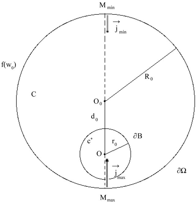
Figure 1. Position of cell .
.
5. Acknowledgements
I want to thank the CNRS Federation “Francilienne de Mecanique, Materiaux Structures et Procedes” CNRS FR2609, in particularly Prof. Didier Clouteau, for financial support in this study.
REFERENCES
- J. Lee and G. Uhlmann, Communications on Pure and Applied Mathematics, Vol. 42, 1989, pp. 1097-1112. doi:10.1002/cpa.3160420804
- D. C. Barber and B. H. Brown, Journal of Physics E: Scientific Instruments, Vol. 17, 1984, pp. 723-733. doi:10.1088/0022-3735/17/9/002
- M. E. Taylor, “Pseudodifferential Operators,” Princeton University Press, Princeton, 1996.
- A. Greenleaf and G. Uhlmann, Duke Mathematical Journal, Vol. 108, 2001, pp. 599-617. doi:10.1215/S0012-7094-01-10837-5
- B. Sapoval, Physical Review Letters, Vol. 73, 1994, pp. 3314-3316. doi:10.1103/PhysRevLett.73.3314
- D. S. Grebenkov, M. Filoche and B. Sapoval, Physical Review E, Vol. 73, 2006, Article ID: 021103. doi:10.1103/PhysRevE.73.021103
- M. E. Taylor, “Partial Differential Equations II: Qualitative Studies of Linear Equations,” Springer-Verlag, Berlin, 1996. doi:10.1007/978-1-4757-4187-2
- J. K. Hunter and B. Nachtergaele, “Applied Analysis,” World Scientific, Singapore City, 2001.
- D. Tataru, Communications in Partial Differential Equations, Vol. 20, 1995, pp. 855-884.
- I. Baydoun, “Opérateurs de Dirichlet-Neumann et Leurs Applications: Transport Laplacien, Problème Inverse et Opérateur de Dirichlet-Neumann,” Éditions Universitaires Européennes, 2012.
- I. Baydoun and V. A. Zagrebnov, Theoretical and Mathematical Physics, Vol. 168, 2011, pp. 1180-1191. doi:10.1007/s11232-011-0097-8
NOTES
1i is the complex number.