Journal of Modern Physics
Vol. 3 No. 9A (2012) , Article ID: 23044 , 20 pages DOI:10.4236/jmp.2012.329145
To the Theory of Galaxies Rotation and the Hubble Expansion in the Frame of Non-Local Physics
Moscow Lomonosov State University of Fine Chemical Technologies, Prospekt Vernadskogo, Moscow, Russia
Email: Boris.Vlad.Alexeev@gmail.com
Received May 4, 2012; revised June 9, 2012; accepted June 17, 2012
Keywords: Dark Matter; Dark Energy; Galaxy: Halo; Galaxy: Kinematics and Dynamics; Hubble Expansion; Hydrodynamics
ABSTRACT
The unified generalized non-local theory is applied for mathematical modeling of cosmic objects. For the case of galaxies the theory leads to the flat rotation curves known from observations. The transformation of Kepler’s regime into the flat rotation curves for different solitons is shown. The Hubble expansion with acceleration is explained as result of mathematical modeling based on the principles of non-local physics. Peculiar features of the rotational speeds of galaxies and effects of the Hubble expansion need not in the introduction of new essence like dark matter and dark energy. The origin of difficulties consists in the total Oversimplification following from the principles of local physics.
1. Introduction
More than ten years ago, the accelerated cosmological expansion was discovered in direct astronomical observations at distances of a few billion light years, almost at the edge of the observable Universe. This acceleration should be explained because mutual attraction of cosmic bodies is only capable of decelerating their scattering. It means that we reach the revolutionary situation not only in physics but also in the natural philosophy on the whole. Practically we are in front of the new challenge since Newton’s Mathematical Principles of Natural Philosophy was published. As result, new idea was introduced in physics about existing of a force with the opposite sign, which is called universal antigravitation. Its physical source is called as dark energy that manifests itself only because of postulated property of providing antigravitation.
It was postulated that the source of antigravitation is “dark matter” which inferred to exist from gravitational effects on visible matter. However, from the other side dark matter is undetectable by emitted or scattered electromagnetic radiation. It means that new essences—dark matter, dark energy—were introduced in physics only with the aim to account for discrepancies between measurements of the mass of galaxies, clusters of galaxies and the entire universe made through dynamical and general relativistic means, measurements based on the mass of the visible “luminous” matter. It could be reasonable if we are speaking about small corrections to the system of knowledge achieved by mankind to the time we are living. But mentioned above discrepancies lead to affirmation, that dark matter constitutes 80% of the matter in the Universe, while ordinary matter makes up only 20%.
Dark matter was postulated by Swiss astrophysicist Fritz Zwicky of the California Institute of Technology in 1933. He applied the virial theorem to the Coma cluster of galaxies and obtained evidence of unseen mass. Zwicky estimated the cluster’s total mass based on the motions of galaxies near its edge and compared that estimate to one based on the number of galaxies and total brightness of the cluster. He found that there was about 400 times more estimated mass than was visually observable. The gravity of the visible galaxies in the cluster would be far too small for such fast orbits, so something extra was required. This is known as the “missing mass problem”. Based on these conclusions, Zwicky inferred that there must be some non-visible form of matter, which would provide enough of the mass, and gravity to hold the cluster together.
The work by Vera Rubin (see for example [1,2]) revealed distant galaxies rotating so fast that they should fly apart. Outer stars rotated at essentially the same rate as inner ones (~254 km/s). This is in marked contrast to the solar system where planets orbit the sun with velocities that decrease as their distance from the centre increases. By the early 1970s, flat rotation curves were routinely detected. It was not until the late 1970s, however, that the community was convinced of the need for dark matter halos around spiral galaxies. The mathematical modeling (based on Newtonian mechanics and local physics) of the rotation curves of spiral galaxies was realized for the various visible components of a galaxy (the bulge, thin disk, and thick disk). These models were unable to predict the flatness of the observed rotation curve beyond the stellar disk. The inescapable conclusion, assuming that Newton’s law of gravity (and the local physics description) holds on cosmological scales, that the visible galaxy was embedded in a much larger dark matter (DM) halo, which contributes roughly 50% - 90% of the total mass of a galaxy. As result another models of gravitation were involved in consideration—from “improved” Newtonian laws (such as modified Newtonian dynamics and tensorvector-scalar gravity [3]) to the Einstein’s theory based on the cosmological constant [4]. Einstein introduced this term as a mechanism to obtain a stable solution of the gravitational field equation that would lead to a static Universe, effectively using dark energy to balance gravity.
Computer simulations with taking into account the hypothetical DM in the local hydrodynamic description include usual moment equations plus Poisson equation with different approximations for the density of DM  containing several free parameters. Computer simulations of cold dark matter (CDM) predict that CDM particles ought to coalesce to peak densities in galactic cores. However, the observational evidence of star dynamics at inner galactic radii of many galaxies, including our own Milky Way, indicates that these galactic cores are entirely devoid of CDM. No valid mechanism has been demonstrated to account for how galactic cores are swept clean of CDM. This is known as the “cuspy halo problem”. As result, the restricted area of CDM influence introduced in the theory. As we see the concept of DM leads to many additional problems.
I do not intend to review the different speculations based on the principles of local physics. I see another problem. It is the problem of Oversimplification—but not “trivial” simplification of the important problem. The situation is more serious—total Oversimplification based on principles of local physics, and obvious crisis, we see in astrophysics, simply reflects the general shortcomings of the local kinetic transport theory. It is important to underline that we should have expected this crisis of local statistical physics after the discovery of Bell’s fundamental inequalities [5]. The antigravitation problem in application to the theory of galaxies rotation and the Hubble expansion is solved further in the frame of non-local statistical physics and the Newtonian law of gravitation.
I deliver here some main ideas and deductions of the generalized Boltzmann physical kinetics and non-local physics. For simplicity, the fundamental methodic aspects are considered from the qualitative standpoint of view avoiding excessively cumbersome formulas. A rigorous description can be found, for example, in the monograph [6].
In 1872 L. Boltzmann [7,8] published his kinetic equation for the one-particle distribution function (DF) . He expressed the equation in the form
 , (1)
, (1)
where  is the local collision integral, and
  is the substantial (particle) derivative,
  and
and  being the velocity and radius vector of the particle, respectively. Boltzmann Equation (1) governs the transport processes in a one-component gas, which is sufficiently rarefied that only binary collisions between particles are of importance and valid only for two character scales, connected with the hydrodynamic time-scale and the time-scale between particle collisions. While we are not concerned here with the explicit form of the collision integral, note that it should satisfy conservation laws of point-like particles in binary collisions. Integrals of the distribution function (i.e. its moments) determine the macroscopic hydrodynamic characteristics of the system, in particular the number density of particles
  and the temperature
 . The Boltzmann equation (BE) is not of course as simple as its symbolic form above might suggest, and it is in only a few special cases that it is amenable to a solution. One example is that of a maxwellian distribution in a locally, thermodynamically equilibrium gas in the event when no external forces are present. In this case the equality
  and
and  is met, giving the maxwellian distribution function
 . A weak point of the classical Boltzmann kinetic theory is the way it treats the dynamic properties of interacting particles. On the one hand, as the so-called “physical” derivation of the BE suggests, Boltzmann particles are treated as material points; on the other hand, the collision integral in the BE brings into existence the cross sections for collisions between particles. A rigorous approach to the derivation of the kinetic equation for
  (noted in following as
 ) is based on the hierarchy of the BogolyubovBorn-Green-Kirkwood-Yvon (BBGKY) [6,9-13] equations.
A  obtained by the multi-scale method turns into the BE if one ignores the change of the distribution function (DF) over a time of the order of the collision time (or, equivalently, over a length of the order of the particle interaction radius). It is important to note [6,14] that accounting for the third of the scales mentioned above leads (prior to introducing any approximation destined to break the Bogolyubov chain) to additional terms, generally of the same order of magnitude, appear in the BE. If the correlation functions is used to derive
  from the BBGKY equations, then the passage to the BE means the neglect of non-local effects.
Given the above difficulties of the Boltzmann kinetic theory, the following clearly inter related questions arise. First, what is a physically infinitesimal volume and how does its introduction (and, as the consequence, the unavoidable smoothing out of the DF) affect the kinetic equation? This question can be formulated in (from the first glance) the paradox form—what is the size of the point in the physical system? Second, how does a systematic account for the proper diameter of the particle in the derivation of the  affect the Boltzmann equation? In the theory developed here, I shall refer to the corresponding
  as Generalized Boltzmann Equation (GBE). The derivation of the GBE and the applications of GBE are presented, in particular, in [6]. Accordingly, our purpose is first to explain the essence of the physical generalization of the BE.
Let a particle of finite radius be characterized, as before, by the position vector  and velocity
  of its center of mass at some instant of time
 . Let us introduce physically small volume (PhSV) as element of measurement of macroscopic characteristics of physical system for a point containing in this PhSV. We should hope that PhSV contains sufficient particles
  for statistical description of the system. In other words, a net of physically small volumes covers the whole investigated physical system.
Every PhSV contains entire quantity of point-like Boltzmann particles, and the same DF  is prescribed for whole PhSV in Boltzmann physical kinetics. Therefore, Boltzmann particles are fully “packed” in the reference volume. Let us consider two adjoining physically small volumes
  and
and . We have in principle another situation for the particles of finite size moving in physical small volumes, which are open thermodynamic systems.
Then, the situation is possible where, at some instant of time t, the particle is located on the interface between two volumes. In so doing, the lead effect is possible (say, for ), when the center of mass of particle moving to the neighboring volume
  is still in
 . However, the delay effect takes place as well, when the center of mass of particle moving to the neighboring volume (say,
 ) is already located in
  but a part of the particle still belongs to
![]() .
.
Moreover, even the point-like particles (starting after the last collision near the boundary between two mentioned volumes) can change the distribution functions in the neighboring volume. The adjusting of the particles dynamic characteristics for translational degrees of freedom takes several collisions. As result, we have in the definite sense “the Knudsen layer” between these volumes. This fact unavoidably leads to fluctuations in mass and hence in other hydrodynamic quantities. Existence of such “Knudsen layers” is not connected with the choice of space nets and fully defined by the reduced description for ensemble of particles of finite diameters in the conceptual frame of open physically small volumes, therefore—with the chosen method of measurement.
This entire complex of effects defines non-local effects in space and time. The corresponding situation is typical for the theoretical physics—we could remind about the role of probe charge in electrostatics or probe circuit in the physics of magnetic effects.
Suppose that DF  corresponds to
  and DF
  is connected with
  for Boltzmann particles. In the boundary area in the first approximation, fluctuations will be proportional to the mean free path (or, equivalently, to the mean time between the collisions). Then for PhSV the correction for DF should be introduced as
 (2)
(2)
in the left hand side of classical BE describing the translation of DF in phase space. As the result
 , (3)
, (3)
where  is the Boltzmann local collision integral.
Important to notice that it is only qualitative explanation of GBE derivation obtained earlier (see for example [6]) by different strict methods from the BBGKY—chain of kinetic equations. The structure of the  is generally as follows
 , (4)
, (4)
where  is the non-local integral term incorporating the non-local time and space effects. The generalized Boltzmann physical kinetics, in essence, involves a local approximation
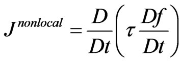 (5)
(5)
for the second collision integral, here in the simplest case  being the mean time between the particle collisions. We can draw here an analogy with the BhatnagarGross-Krook (BGK) approximation for
 ,
,
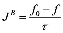 , (6)
, (6)
which popularity as a means to represent the Boltzmann collision integral is due to the huge simplifications it offers. In other words—the local Boltzmann collision integral admits approximation via the BGK algebraic expression, but more complicated non-local integral can be expressed as differential form (5). The ratio of the second to the first term on the right-hand side of Equation (4) is given to an order of magnitude as 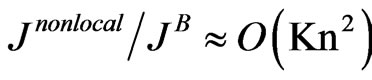 and at large Knudsen numbers (Kn defining as ratio of mean free path of particles to the character hydrodynamic length) these terms become of the same order of magnitude. It would seem that at small Knudsen numbers answering to hydrodynamic description the contribution from the second term on the right-hand side of Equation (4) is negligible.
This is not the case, however. When one goes over to the hydrodynamic approximation (by multiplying the kinetic equation by collision invariants and then integrating over velocities), the Boltzmann integral part vanishes, and the second term on the right-hand side of Equation (4) gives a single-order contribution in the generalized Navier-Stokes description. Mathematically, we cannot neglect a term with a small parameter in front of the higher derivative. Physically, the appearing additional terms are due to viscosity and they correspond to the small-scale Kolmogorov turbulence [6,15]. The integral term  turns out to be important both at small and large Knudsen numbers in the theory of transport processes. Thus,
  is the distribution function fluctuation, and writing Equation (3) without taking into account Equation (2) makes the BE non-closed. From viewpoint of the fluctuation theory, Boltzmann employed the simplest possible closure procedure
 .
.
Then, the additional GBE terms (as compared to the BE) are significant for any Kn, and the order of magnitude of the difference between the BE and GBE solutions is impossible to tell beforehand. For GBE the generalized H-theorem is proven [6,16].
It means that the local Boltzmann equation does not belong even to the class of minimal physical models and corresponds so to speak to “the likelihood models”. This remark refers also to all consequences of the Boltzmann kinetic theory including “classical” hydrodynamics.
Obviously the generalized hydrodynamic equations (GHE) will explicitly involve fluctuations proportional to . In the hydrodynamic approximation, the mean time
  between the collisions is related to the dynamic viscosity
  by
by
 , (7)
, (7)
[17,18]. For example, the continuity equation changes its form and will contain terms proportional to viscosity. On the other hand, if the reference volume extends over the whole cavity with the hard walls, then the classical conservation laws should be obeyed, and this is exactly what the monograph [6] proves. Now several remarks of principal significance:
1) All fluctuations are found from the strict kinetic considerations and tabulated [6]. The appearing additional terms in GHE are due to viscosity and they correspond to the small-scale Kolmogorov turbulence. The neglect of formally small terms is equivalent, in particular, to dropping the (small-scale) Kolmogorov turbulence from consideration and is the origin of all principal difficulties in usual turbulent theory. Fluctuations on the wall are equal to zero, from the physical point of view this fact corresponds to the laminar sub-layer. Mathematically it leads to additional boundary conditions for GHE. Major difficulties arose when the question of existence and uniqueness of solutions of the Navier-Stokes equations was addressed.
O. A. Ladyzhenskaya has shown for three-dimensional flows that under smooth initial conditions a unique solution is only possible over a finite time interval. Ladyzhenskaya even introduced a “correction” into the NavierStokes equations in order that its unique solvability could be proved (see discussion in [19]). GHE do not lead to these difficulties.
2) It would appear that in continuum mechanics the idea of discreteness can be abandoned altogether and the medium under study be considered as a continuum in the literal sense of the word. Such an approach is of course possible and indeed leads to the Euler equations in hydrodynamics. However, when the viscosity and thermal conductivity effects are to be included, a totally different situation arises. As is well known, the dynamical viscosity is proportional to the mean time  between the particle collisions, and a continuum medium in the Euler model with
  implies that neither viscosity nor thermal conductivity is possible.
3) The non-local kinetic effects listed above will always be relevant to a kinetic theory using one particle description—including, in particular, applications to liquids or plasmas, where self-consistent forces with appropriately cut-off radius of their action are introduced to expand the capability of GBE [20-25]. Fluctuation effects occur in any open thermodynamic system bounded by a control surface transparent to particles. GBE (3) leads to generalized hydrodynamic equations [6] as the local approximation of non local effects, for example, to the continuity equation
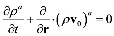 , (8)
, (8)
where ,
,  ,
,  are calculated in view of nonlocality effect in terms of gas density
 , hydrodynamic velocity of flow
 , and density of momentum flux
 ; for locally Maxwellian distribution,
  ,
,  are defined by the relations
 , (9)
, (9)
where  is a unit tensor, and
  is the acceleration due to the effect of mass forces.
In the general case, the parameter  is the non-locality parameter; in quantum hydrodynamics, the “timeenergy” uncertainty relation defines its magnitude. The violation of Bell’s inequalities [5] is found for local statistical theories, and the transition to non-local description is inevitable. The following conclusion of principal significance can be done from the generalized quantum consideration [22,23]:
1) Madelung’s quantum hydrodynamics is equivalent to the Schrödinger equation (SE) and leads to description of the quantum particle evolution in the form of Euler equation and continuity equation.
2) SE is consequence of the Liouville equation as result of the local approximation of non-local equations.
3) Generalized Boltzmann physical kinetics defines the strict approximation of non-local effects in space and time and after transmission to the local approximation leads to parameter , which on the quantum level corresponds to the uncertainty principle “time-energy”.
4) GHE lead to SE as a deep particular case of the generalized Boltzmann physical kinetics and therefore of non-local hydrodynamics.
In principal GHE needn’t in using of the “time-energy” uncertainty relation for estimation of the value of the non-locality parameter . Moreover, the “time-energy” uncertainty relation does not lead to the exact relations and from position of non-local physics is only the simplest estimation of the non-local effects.
Really, let us consider two neighboring physically infinitely small volumes  and
and  in a nonequilibrium system. Obviously the time
  should tend to diminish with increasing of the velocities
  of particles invading in the nearest neighboring physically infinitely small volume (
 or
or ):
):
 . (10)
However, the value  cannot depend on the velocity direction and naturally to tie
  with the particle kinetic energy, then
 (11)
(11)
where  is a coefficient of proportionality, which reflects the state of physical system. In the simplest case
  is equal to Plank constant
  and relation (11) becomes compatible with the Heisenberg relation.
Finally, we can state that introduction of open control volume by the reduced description for ensemble of particles of finite diameters leads to fluctuations (proportional to Knudsen number) of velocity moments in the volume. This fact defines the significant reconstruction of the theory of transport processes. Obviously the mentioned non-local effects can be discussed from viewpoint of breaking of the Bell’s inequalities [5] because in the non-local theory the measurement (realized in ) has influence on the measurement realized in the adjoining space-time point in
  and verse versa.
In the following sections I intend to apply the unified generalized non-local theory for mathematical modeling of cosmic objects. For the case of galaxies the theory leads to the flat rotation curves known from observations. The transformation of Kepler’s regime into the flat rotation curves for different solitons is shown. The Hubble expansion with acceleration is explained as result of mathematical modeling based on the principals of nonlocal physics. Therefore the answers for the following questions are formulated:
1) Why the concept of the dark matter is not significant in the Solar system?
2) Why the galaxy rotation curves have the character flat form?
3) Is it possible to obtain the continuous transition from the Kepler regime to the flat halo curves?
4) Why after Big Bang explosion (or after the explosion in the Hubble boxes) the Hubble expansion exists with acceleration? ([26-28], Nobel Prize for the observers S. Perlmutter, A. G. Riess, B. Schmidt of the year 2011).
In other words—is it possible using only Newtonian gravitation law and non-local statistical description to forecast the flat gravitational curve of a typical spiral galaxy (Section 2) and the Hubble expansion (including the Hubble expansion with acceleration, PRS-regime), (Section 3)? The last question has the positive answer.
0B2. Disk Galaxy Rotation and the Problem of Dark MatterAbout forty years after Zwicky’s initial observations Vera Rubin, astronomer at the Department of Terrestrial Magnetism at the Carnegie Institution of Washington presented findings based on a new sensitive spectrograph that could measure the velocity curve of edge-on spiral galaxies to a greater degree of accuracy than had ever before been achieved. Together with Kent Ford, Rubin announced at a 1975 meeting of the American Astronomical Society the astonishing discovery that most stars in spiral galaxies orbit at roughly the same speed reflected schematically on Figure 1.
For example, the rotation curve of the type B corresponds to the galaxy NGC3198. The following extensive radio observations determined the detailed rotation curve of spiral disk galaxies to be flat (as the curve B), much beyond as seen in the optical band. Obviously the trivial balance between the gravitational and centrifugal forces leads to relation between orbital speed  and galactocentric distance
  as
as  beyond the physical extent of the galaxy of mass
  (the curve A).
Figure 1. Rotation curve of a typical spiral galaxy: predicted (A) and observed (B).
The obvious contradiction with the velocity curve B having a “flat” appearance out to a large radius, was explained by introduction of a new physical essence—dark matter because for spherically symmetric case the hypothetical density distribution  leads to
 . The result of this activity is known—undetectable dark matter which does not emit radiation, inferred solely from its gravitational effects. But it means that upwards of 50% of the mass of galaxies was contained in the dark galactic halo.
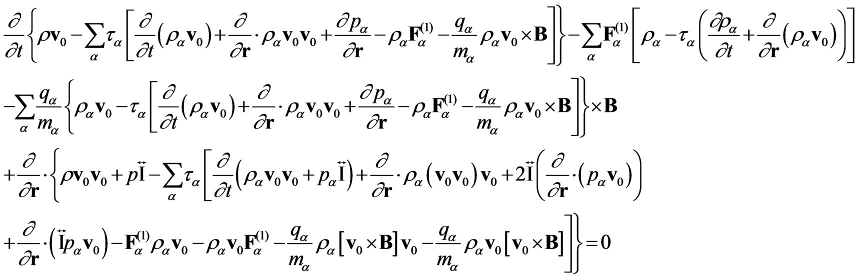
Strict consideration leads to the following system of the generalized hydrodynamic equations (GHE) [6,22-25, 29-31] written in the generalized Euler form:
(Continuity equation for species ![]() )
)
 (12)
(12)
(Continuity equation for mixture)
 (13)
(13)
(Momentum equation for species )
)
 (14)
(14)
(Momentum equation for mixture)
 (15)
(15)
(Energy equation for  species)
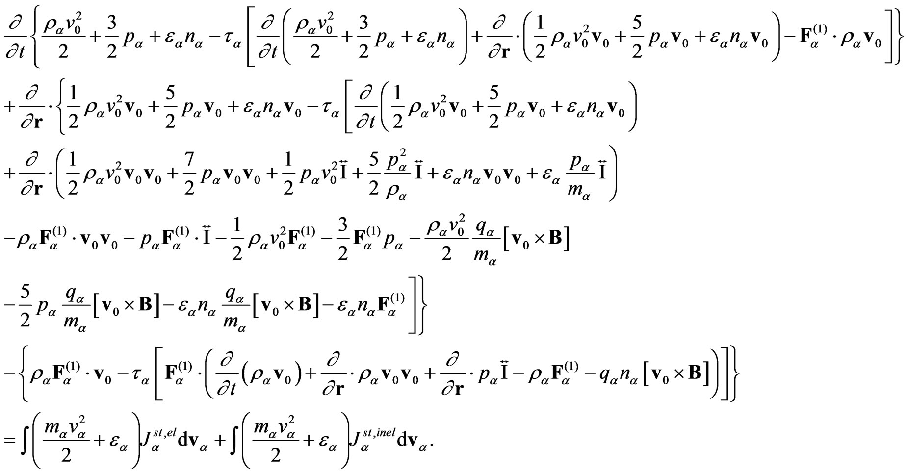 (16)
(16)
(Energy equation for mixture)
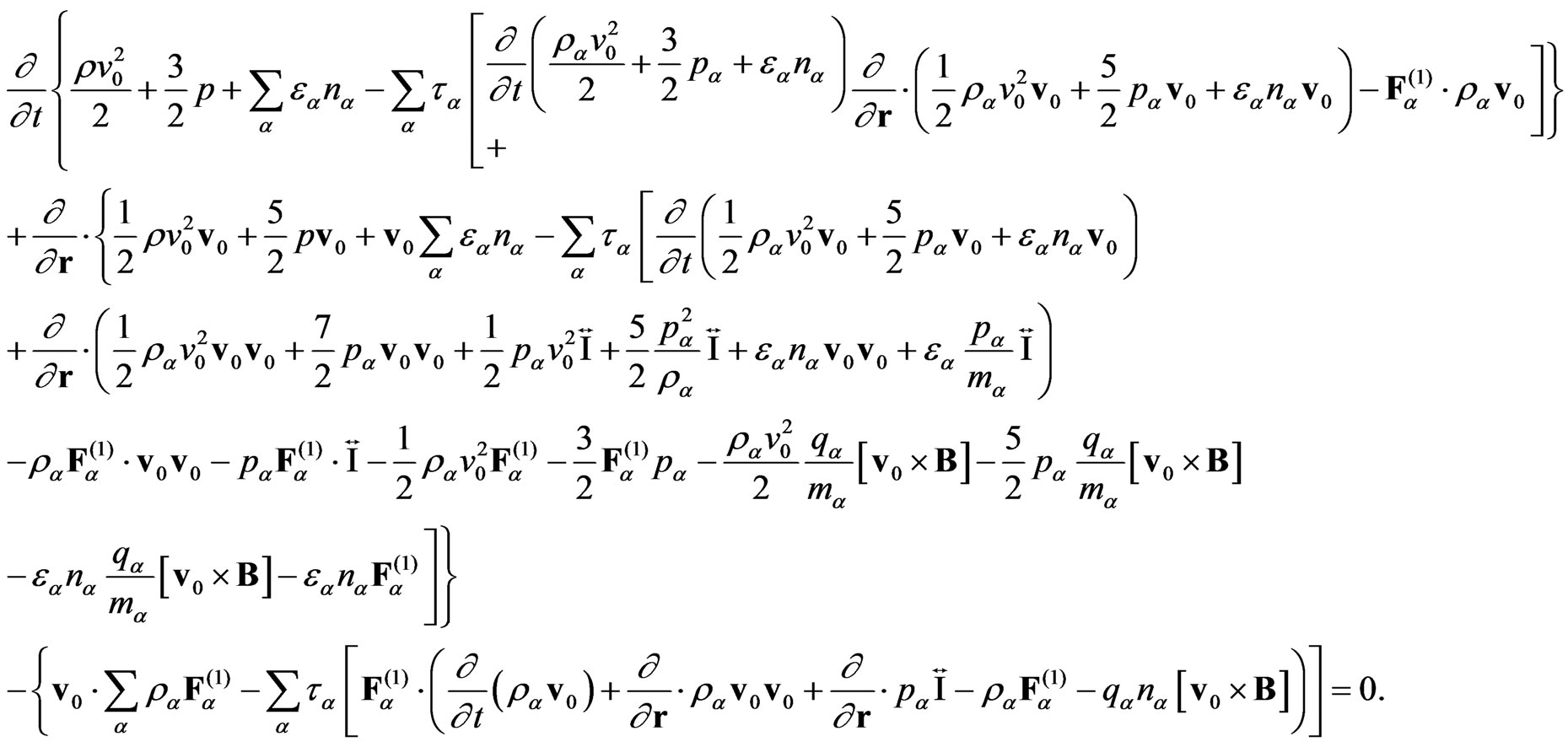 (17)
(17)
Here  are the forces of the non-magnetic origin,
 —magnetic induction,
 —unit tensor,
 —charge of the α-component particle,
 —static pressure for α-component,
 —internal energy for the particles of α-component,
 — hydrodynamic velocity for mixture,
 —non-local parameter.
GHE can be applied to the physical systems from the Universe to atomic scales. All additional explanations will be done by delivering the results of modeling of corresponding physical systems with the special consideration of non-local parameters . Generally speaking to GHE should be added the system of generalized Maxwell equations (for example in the form of the generalized Poisson equation for electric potential) and gravitational equations (for example in the form of the generalized Poisson equation for gravitational potential).
In the following I intend to show that the character features reflected on Figure 1 can be explained in the frame of Newtonian gravitation law and the non-local kinetic description created by me. With this aim let us consider the formation of the soliton’s type of solution of the generalized hydrodynamic equations for gravitational media like galaxy in the self consistent gravitational field. Our aim consists in calculation of the self-consistent hydrodynamic moments of possible formation like gravitational soliton.
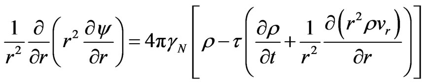
Let us investigate of the gravitational soliton formation in the frame of the non-stationary 1D Cartesian formulation. Then the system of GHE consist from the generalized Poisson equation reflecting the effects of the density and the density flux perturbations, continuity equation, motion and energy equations. The GHE derivation can be found in [6,15,29]. This system of four equations for non-stationary 1D case is written as the deep particular case of Equations (12)-(17) in the form:
(Poisson equation)
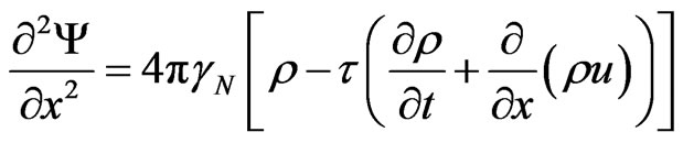 , (18)
(Continuity equation)
 (19)
(19)
(Motion equation)
 (20)
(20)
(Energy equation)
 (21)
(21)
where  is translational velocity of the one species object,
 —self consistent gravitational potential (
 is acceleration in gravitational field),
  is density and
  is pressure,
  is non-locality parameter,
  is Newtonian gravitation constant.
Let us introduce the coordinate system moving along the positive direction of x-axis in ID space with velocity  equal to phase velocity of considering object
 . (22)
Taking into account the De Broglie relation we should wait that the group velocity  is equal 2
 . In moving coordinate system all dependent hydrodynamic values are function of
 . We investigate the possibility of the object formation of the soliton type. For this solution there is no explicit dependence on time for coordinate system moving with the phase velocity
 . Write down the system of Equations (18)-(21) in the dimensionless form, where dimensionless symbols are marked by tildes.
For the scales ,
,  ,
,
 and conditions
 , the equations take the form:
(Generalized Poisson equation)
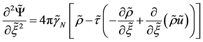 , (23)
(Continuity equation)
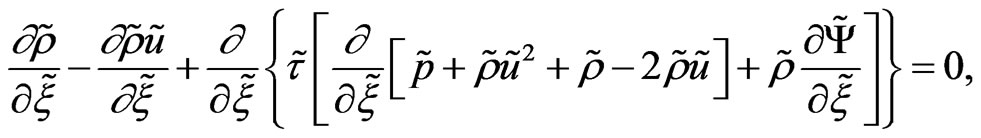 (24)
(24)
(Motion equation)
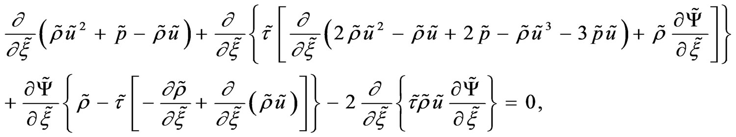 (25)
(25)
(Energy equation)
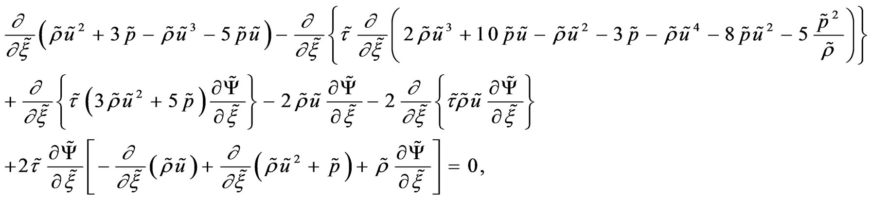 (26)
(26)
Some comments to the system of four ordinary nonlinear Equations (23)-(26):
1) Every equation from the system is of the second order and needs two conditions. The problem belongs to the class of Cauchy problems.
2) In comparison for example, with the Schrödinger theory connected with behavior of the wave function, no special conditions are applied for dependent variables including the domain of the solution existing. This domain is defined automatically in the process of the numerical solution of the concrete variant of calculations.
3) From the introduced scales ,
,  ,
,  , only three parameters are independent, namely,
 .
.
4) Approximation for the dimensionless non-local parameter  should be introduced (see (11)). In the definite sense it is not the problem of the hydrodynamic level of the physical system description (like the calculation of the kinetic coefficients in the classical hydrodynamics). Interesting to notice that quantum GHE were applied with success for calculation of atom structure [22-25], which is considered as two species charged
  mixture. The corresponding approximations for non-local parameters
 ,
,  and
and  are proposed in [22,23]. In the theory of the atom structure [23] after taking into account the Balmer’s relation, (11) transforms into
 , (27)
where  is principal quantum number. As result the length scale relation was written as
 . But the value
has the dimension  and can be titled as quantum viscosity,
 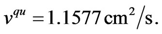 Then
Then
 . (28)
Introduce now the quantum Reynolds number
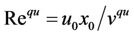 . (29)
As result from (27)-(29) follows the condition of quantization for . Namely
 (30)
(30)
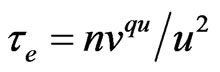
5) Taking into account the previous considerations I introduce the following approximation for the dimensionless non-local parameter
 , (31)
 , (32)
where the scale for the kinematical viscosity is introduced . Then we have the physically transparent result—non-local parameter is proportional to the kinematical viscosity and in inverse proportion to the square of velocity.
The system of generalized hydrodynamic Equations (23)-(26) (solved with the help of Maple) have the great possibilities of mathematical modeling as result of changing of eight Cauchy conditions describing the character features of initial perturbations which lead to the soliton formation. The following Maple notations on figures are used: r—density , u—velocity
 , p— pressure
  and v—self consistent potential
 .
.
Explanations placed under all following figures, Maple program contains Maple’s notations—for example the expression  means in the usual notations
 , independent variable
  responds to
 .
.
We begin with investigation of the problem of principle significance—is it possible after a perturbation (defined by Cauchy conditions) to obtain the gravitational object of the soliton’s kind as result of the self-organization of the matter? With this aim let us consider the initial perturbations (SYSTEM I): ,
,  ,
,  ,
,  ,
,  ,
,  ,
,  ,
, .
.
The Figures 2-4 reflect the result of solution of Equations (23)-(26) with the choice of scales leading to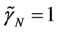 . Figures 2-5 correspond to the approximation of the non-local parameter
  in the form (31). Figure 2
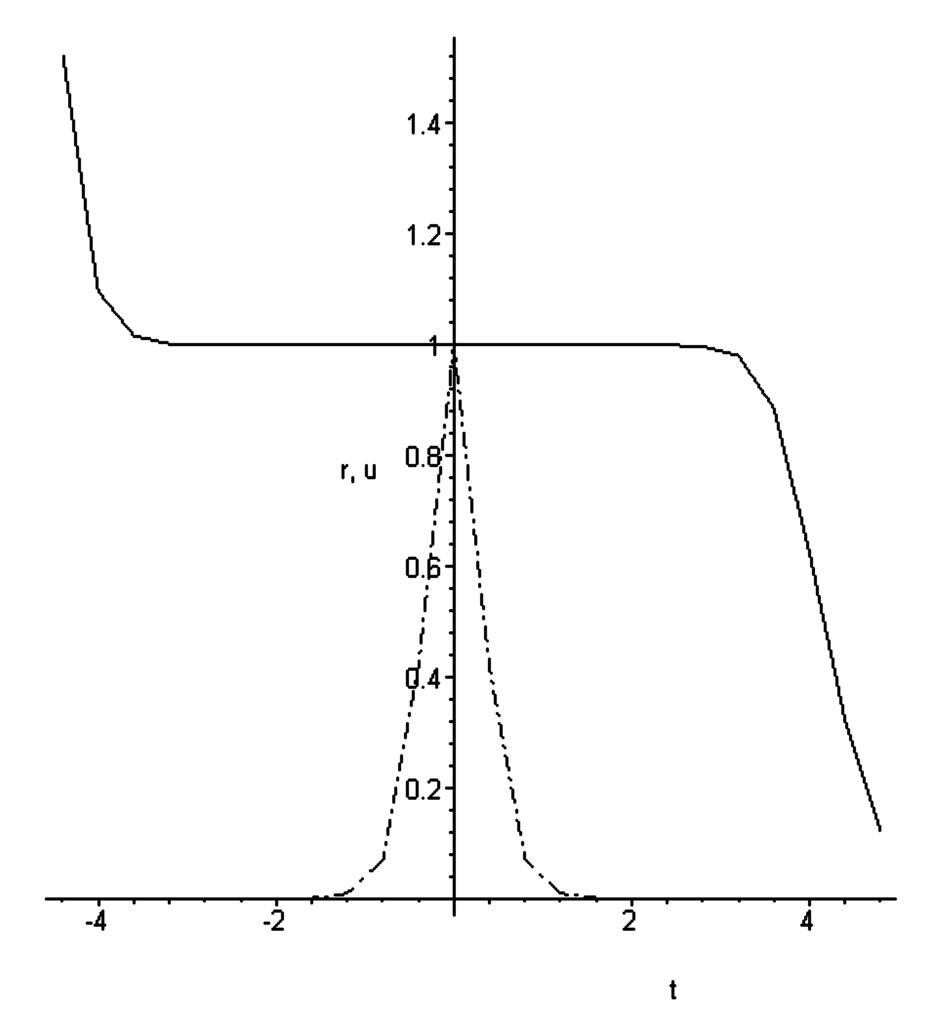
Figure 2. r density  (dash dotted line), u velocity
  in gravitational soliton.
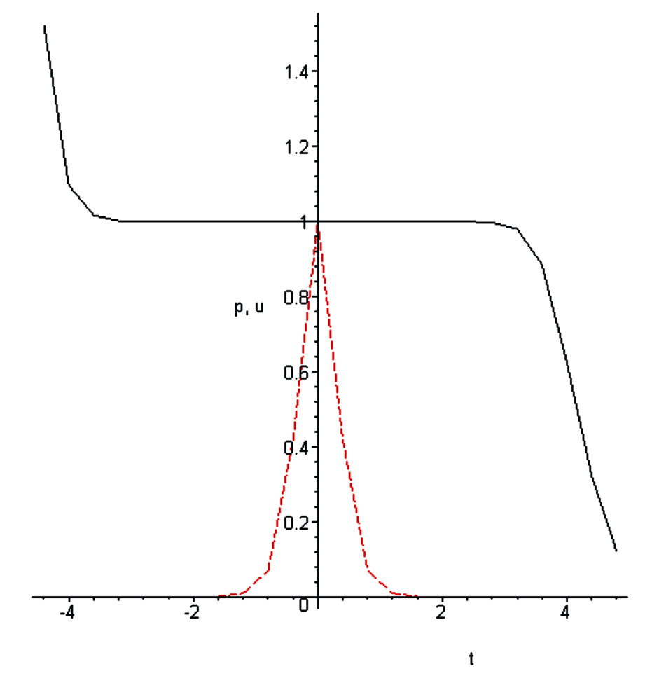
Figure. 3. p pressure  (dashed line), u velocity
  in gravitational soliton.
Figure 4. u velocity , v self consistent potential
 ,
,  in soliton.
displays the gravitational object placed in bounded region of 1D Cartesian space, all parts of this object are moving with the same velocity. Important to underline that no special boundary conditions were used for this and all following cases. Then this soliton is product of the self-organization of gravitational matter. Figures 3 and 4 contain the answer for formulated above question
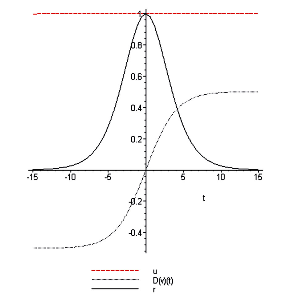
Figure 5. u velocity , r density
 ,
,  in soliton, (
 ).
).
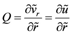
about stability of the object. The derivative (see Figure 4)
 is proportional to the self-consistent gravitational force acting on the soliton and in its vicinity. Therefore the stability of the object is result of the self-consistent influence of the gravitational potential and pressure.
Extremely important that the self-consistent gravitational force has the character of the flat area which exists in the vicinity of the object. This solution exists only in the restricted area of space; the corresponding character length is defined automatically as result of the numerical solution of the problem. The non-local parameter , in the definite sense plays the role analogous to kinetic coefficients in the usual Boltzmann kinetic theory. The influence on the results of calculations is not too significant. The same situation exists in the generalized hydrodynamics. Really, let us use the another approximation for
  in the simplest possible form, namely
 . (33)
The following Figures 6-10 reflect the results of solution of Equations (23)-(26) with the choice of scales leading to , but with the approximation of the non-local parameter
  in the form (33).
Spiral galaxies have rather complicated geometrical forms and 3D calculations can be used. But reasonable to suppose that influence of halo on galaxy kernel is not too significant and to use for calculations the spherical coordinate system. The 1D calculations in the Cartesian
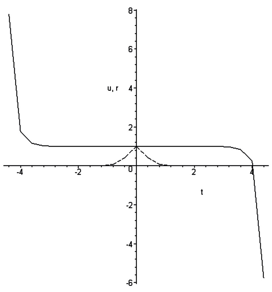
Figure 6. r density  (dashed line), u velocity
  in gravitational soliton.
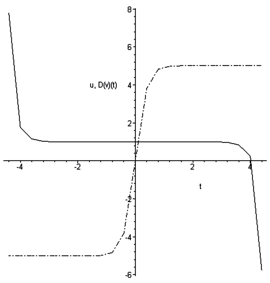
Figure 7. u velocity ,
,  (dash-dotted line).
coordinate system correspond to calculations in the spherecal coordinate system by the large radii of curvature, but have also the independent significance in another character scales. Namely for explanations of the meteorological front motion (without taking into account the Earth rotation). In this theory cyclone or anticyclone corresponds to moving solitons. In the Earth scale the
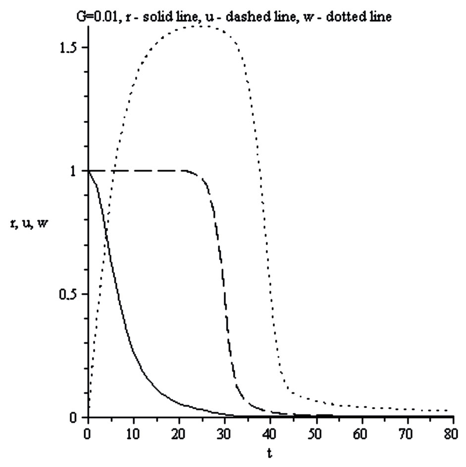
Figure 8. r density , u velocity
 , w orbital velocity
 .
. .
.
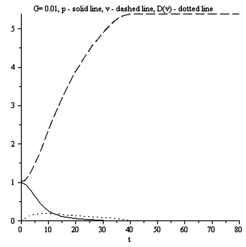
Figure 9. p pressure , v self consistent potential in gravitational soliton,
  ,
,  in gravitational soliton.
scales can be used: ,
,  ,
,  and
and . Figure 5 reflects the results of the corresponding calculation and in particular reflects correctly the wind orientation in front and behind of the soliton.
The full system of 3D non-local hydrodynamic equations in moving (along x axis) Cartesian coordinate system and the corresponding expression for derivatives in
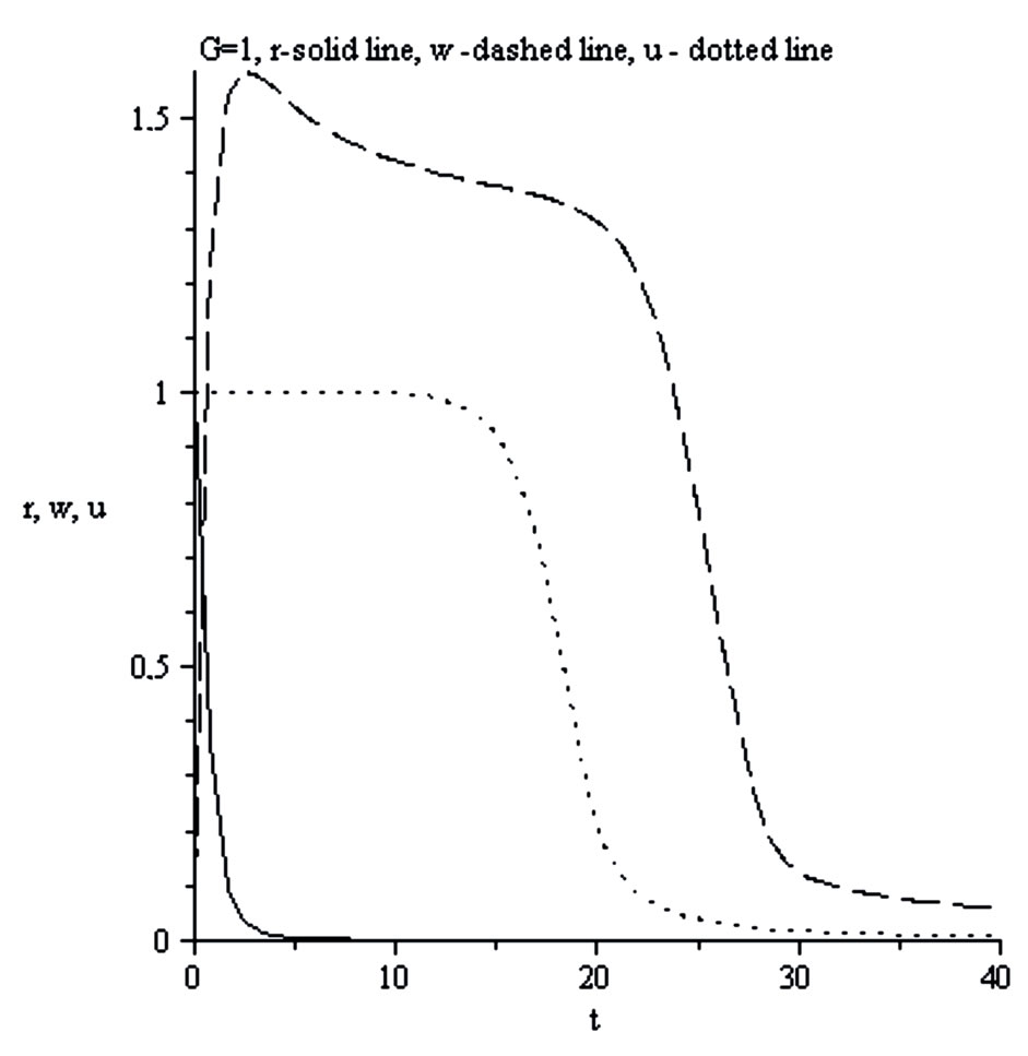
Figure 10. r density , u velocity
  in gravitational soliton, w orbital velocity
 .
. .
.
the spherical coordinate system can be found in [29,30]. The following figures reflect the result of soliton calculations for the case of spherical symmetry for galaxy kernel. The velocity  corresponds to the direction of the soliton movement for spherical coordinate system on following figures. Self-consistent gravitational force
  acting on the unit of mass permits to define the orbital velocity
  of objects in halo,
  , or
, or
 , (34)
where  is the distance from the center of galaxy. All calculations are realized for the conditions (SYSTEM I) but for different parameter
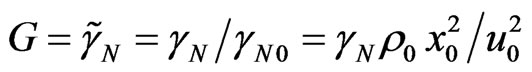 . (35)
Parameter  plays the role of similarity criteria in traditional hydrodynamics. Important conclusions:
1) The following Figures 8-15 demonstrate evolution of the rotation curves from the Kepler regime (Figures 8 and 9; small G, like curve A on Figure 1) to observed (Figures 14 and 15; large G, like curve B on Figure 1) for typical spiral galaxies.
2) The stars with planets (like Sun) correspond to the gravitational soliton with small G and therefore originate the Kepler rotation regime.
3) Regime B cannot be obtained in the frame of local statistical physics in principal and authors of many papers introduce different approximations for additional “dark matter density” (as usual in Poisson equation) trying to find coincidence with data of observations.
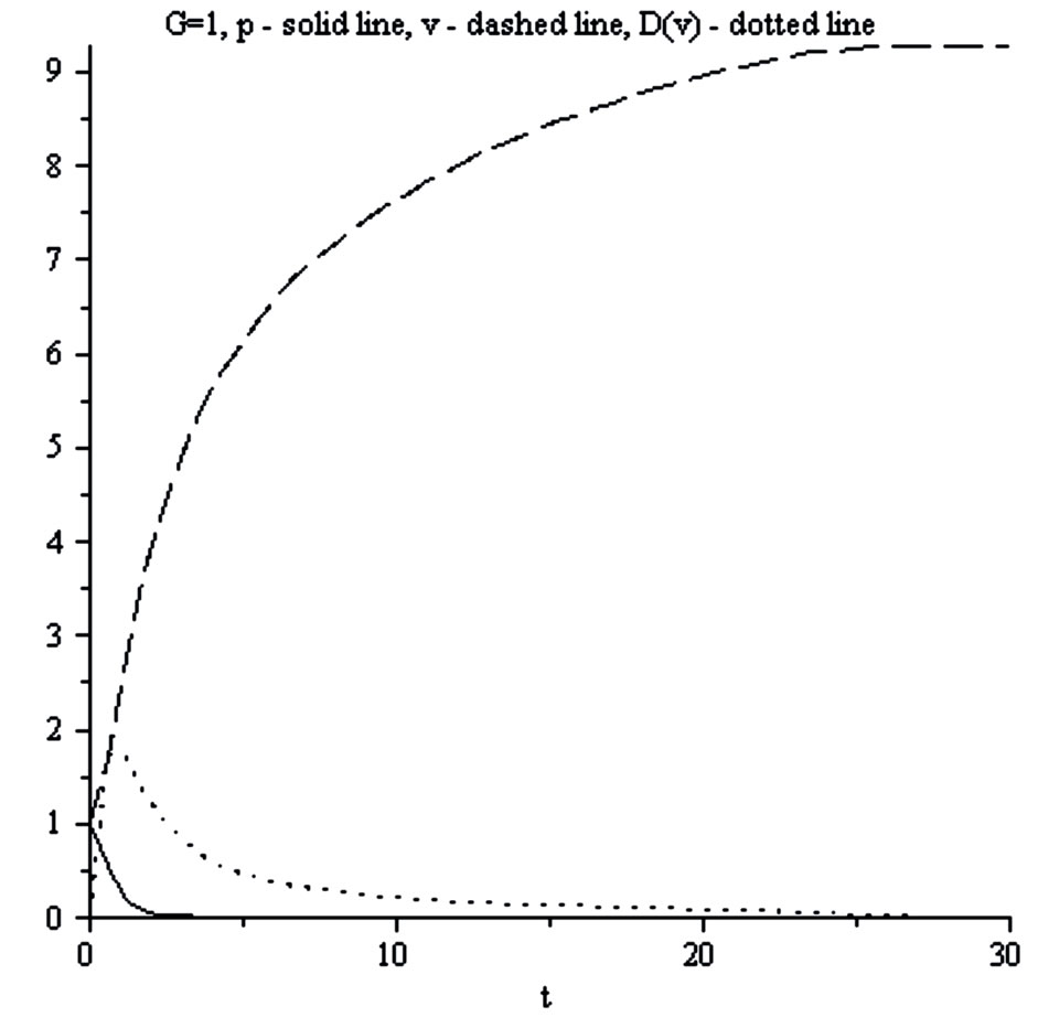
Figure 11. p pressure , v self consistent potential
 ,
,  in gravitational soliton.
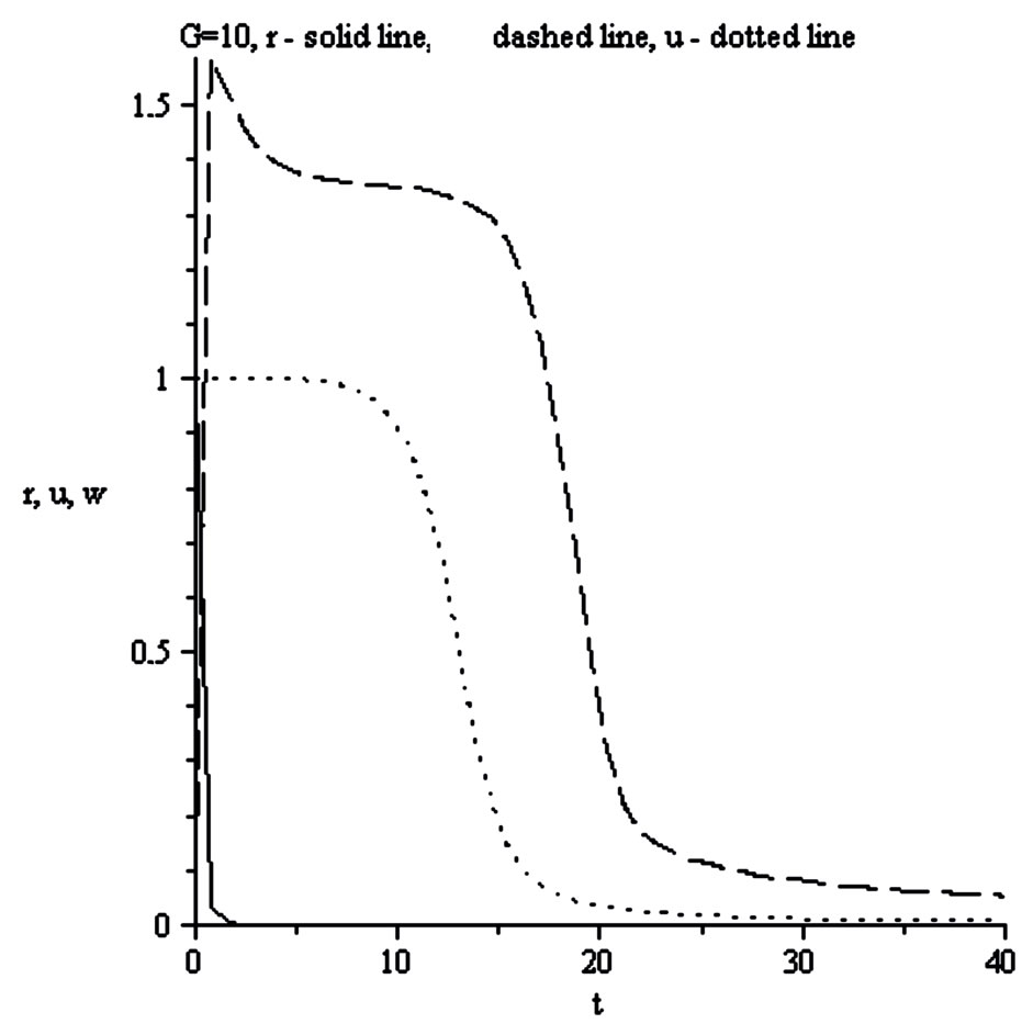
Figure 12. r density , u velocity
  in gravitational soliton, w orbital velocity
 .
. .
.
4) From the wrong position of local theories Poisson Equation (18) contains “dark matter density”, continuity Equation (19) contains the “flux of dark matter density”, motion Equation (20) includes “dark energy”, energy Equation (21) has “the flux of dark energy” and so on to the “senior dark velocity moments”. This entire situation is similar to the turbulent theories based on local statistical physics and empirical corrections for velocity moments.
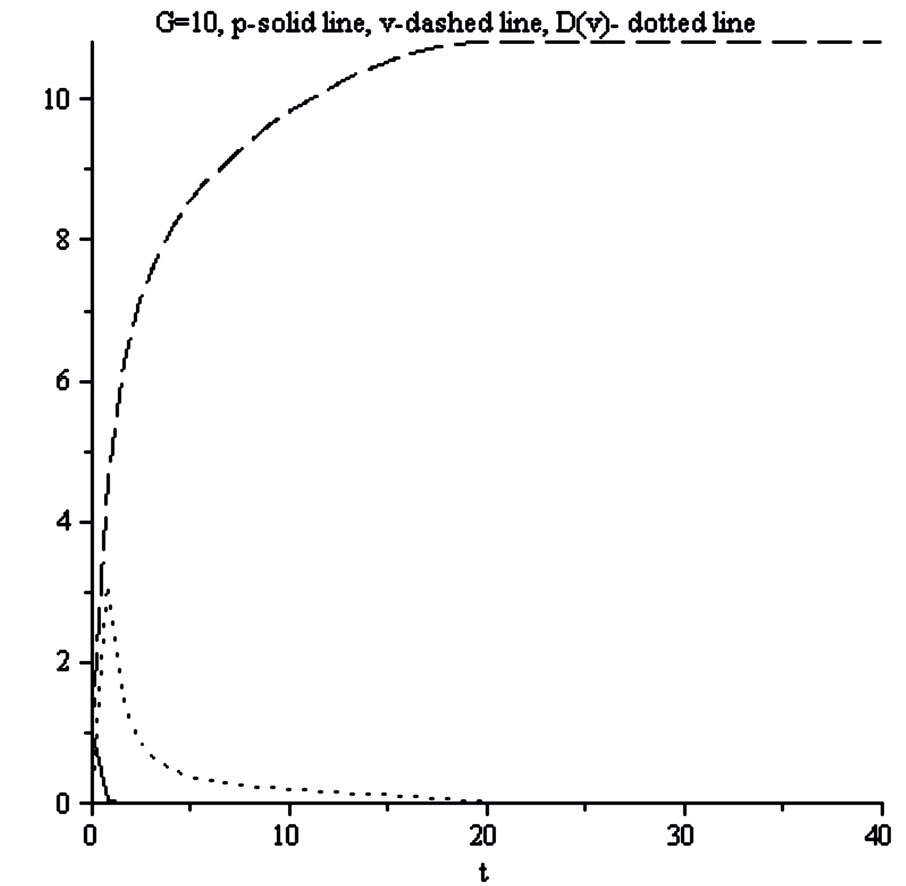
Figure 13. p pressure , v self consistent potential
 ,
, .
.
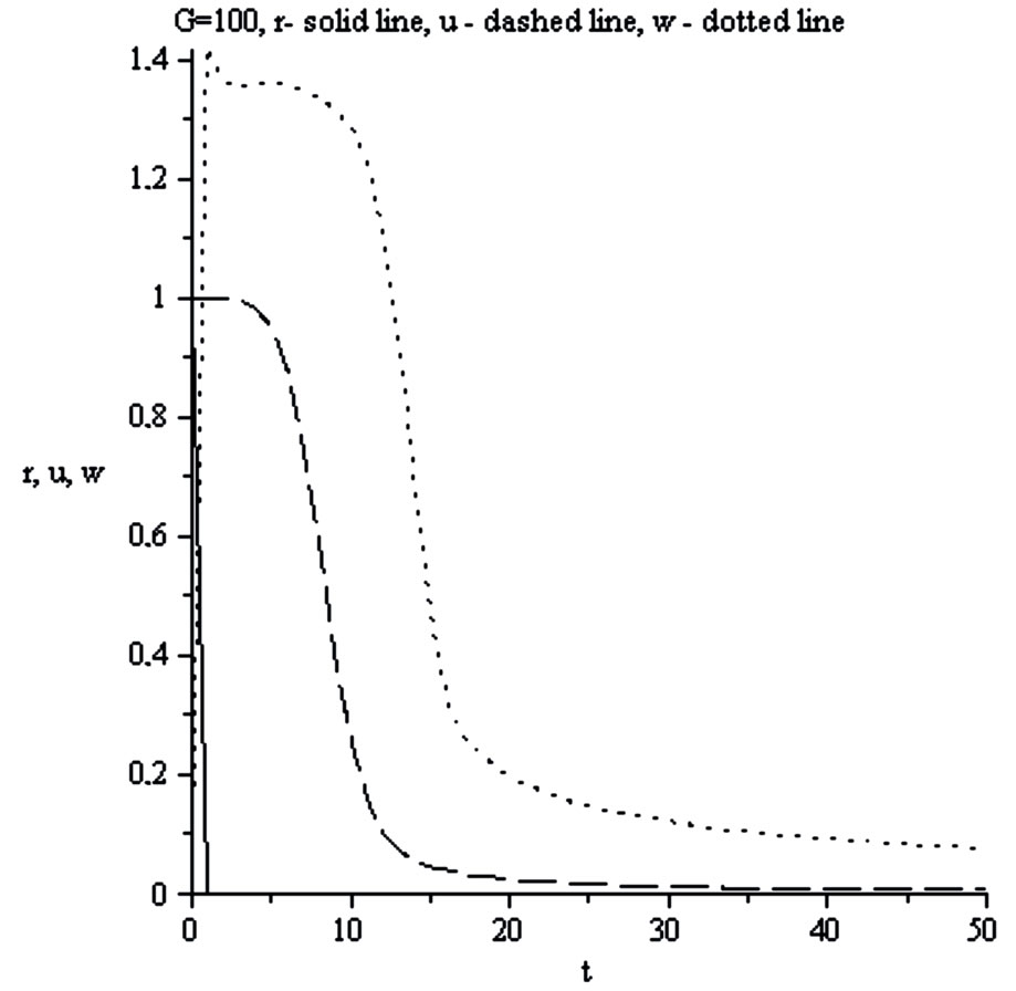
Figure 14. r density , u velocity
  in gravitational soliton, w orbital velocity
 .
. .
.
As we see peculiar features of the halo movement can be explained without new concepts like “dark matter”. Important to underline that the shown transformation of the Kepler’s regime into the flat rotation curves for different solitons explains the “mysterious” fact of the dark matter absence in the Sun vicinity.
3. Hubble Expansion and the Problem of Dark Energy
In simplest interpretation of the local theories the dark
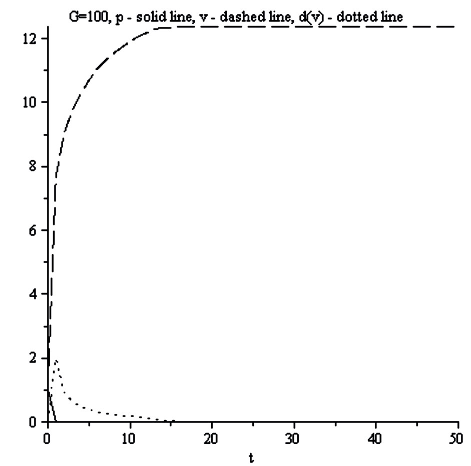
Figure. 15. p pressure , v self consistent potential
 ,
, .
.
energy is related usually to the Einstein cosmological constant. In review [4] the modified Newton force is written as
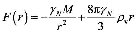 , (36)
where  is the Einstein-Gliner vacuum density [33]. In the limit of large distances the influence of central mass
  becomes negligibly small and the field of forces is determined only by the second term in the right side of (36). It follows from relation (36) that there is a distance
  at which the sum of the gravitation and antigravitation forces is equal to zero. In other words
  is “the zero-gravitational radius”. For so called Local Group of galaxies estimation of
  is about 1Mpc.
From the non-local statistical theory the physical picture follows which leading to the Hubble flow without new essence like dark energy and without modification of Newton force like (36).
Namely:
The main origin of Hubble effect (including the matter expansion with acceleration) is self—catching of expanding matter by the self—consistent gravitational field in conditions of weak influence of the central massive bodies.
The formulated result is obtained in the frame of the linear theory [25,31]. Is it possible to obtain the corresponding result on the level of the general non-linear description? Such an investigation was successfully realized and leads to a direct mathematical model supporting the well known observations of S. Perlmutter, A. Riess (USA) and B. Schmidt (Australia). These researchers studied Type 1a supernovae and determined that more distant galactic objects seem to move faster. Their observations suggest that not only is the Universe expanding, its expansion is relentlessly speeding up.
Effects of gravitational self-catching should be typical for Universe. The existence of “Hubble boxes” is discussed in review [4] as typical blocks of the nearby Universe. Gravitational self-catching takes place for Big Bang having given birth to the global expansion of Universe, but also for Little Bang in so called Local Group (using the Hubble’s terminology) of galaxies. Then the evolution of the Local Group (the typical Hubble box) is really fruitful field for testing of different theoretical constructions (see Figure 16). The data were obtained by Karachentsev and his collaborators in 2002-2007 in observation with the Hubble Space Telescope [4,32]. Each point corresponds to a galaxy with measured values of distance and line-of-site velocity in the reference frame related to the center of the Local Group. The diagram shows two distinct structures, the Local Group and the local flow of galaxies. The galaxies of the Local Group occupy a volume with the radius up to ~1.1 - 1.2 Mpc, but there are no galaxies in the volume whose radius is less than 0.25 Mpc. These galaxies move both away from the center (positive velocities) and toward the center (negative velocities). These galaxies form a gravitationally bound quasi-stationary system. Their average radial velocity is equal to zero. The galaxies of the local flow are located outside the group and all of them are moving from the center (positive velocities) beginning their motion near  with the velocity
 . By the way the measured by Karachentsev the average Hubble parameter for the Local Group is 72 ± 6
 .
.
Let us choose these values as scales:
 . (37)
Recession velocities increase as the distance increases in accordance with the Hubble law. The straight line correspond the dependence from observations
 (38)
(38)
for the region outside of the Local Group. In the nondimensional form
 (39)
(39)
where
 . (40)
For the following calculations we should choose the corresponding scales (especially for estimating ) for modeling of the Local Group evolution
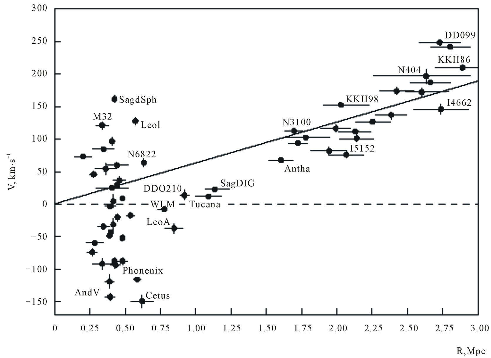
Figure 16. Velocity-distance diagram for galaxies at distances of up to 3 Mpc for local group of galaxies.
 . (41)
For the density scale estimation the average density of the local flow could be used. But the corresponding data are not accessible and I use the average density of the Local Group which can be taken from references [32,34] with . Then from (41) we have
 .
.
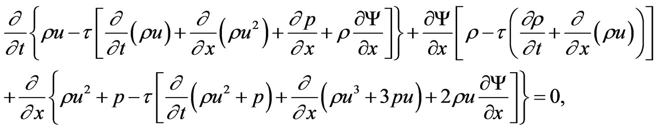
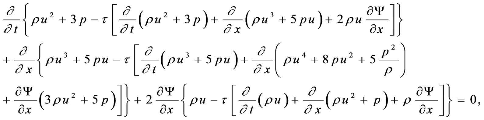
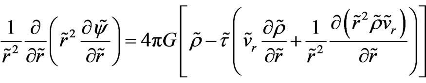
Let us go now to the mathematical modeling. The nonlocal system of hydrodynamic equations describing the explosion with the spherical symmetry is written as (see [30], Appendix 2)
 , (42)
(Poisson equation)
 , (43)
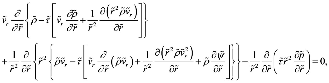
(Continuity equation)
 , (44)
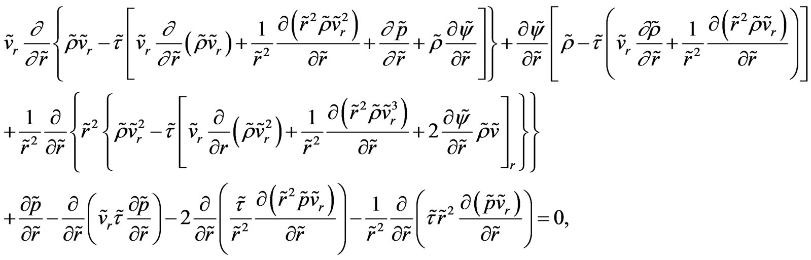
(Motion equation)
 , (45)
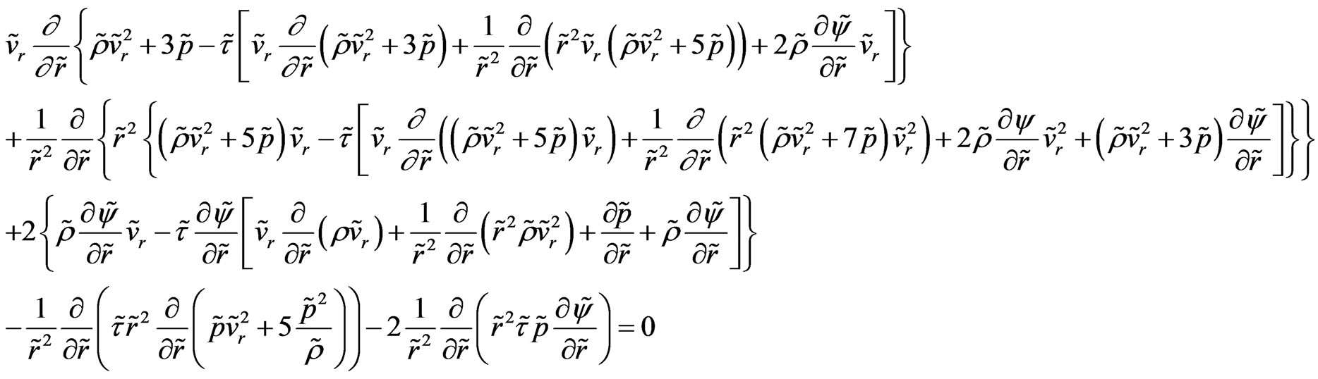
(Energy equation)
 (46)
(46)
The system of Equations (43)-(46) belongs to the class of the 1D non-stationary equations and can be solved by known numerical methods. But for the aims of the transparent vast mathematical modeling of self-catching of the expanding matter by the self-consistent gravitational field I introduce the following assumption. Let us allot the quasi-stationary Hubble regime when only the implicit dependence on time for the unknown values exists. It means that for the intermediate (Hubble) regime the substitution
 (47)
(47)
can be introduced. As result we have the following system of the 1D dimensionless equations:
 ,(48)
,(48)
 (49)
(49)
 (50)
(50)
 (51)
(51)
The system of generalized hydrodynamic equations (48)-(51) have the great possibilities of mathematical modeling as result of changing of eight Cauchy conditions describing the character features of the local flow evolution. The following Maple notations on figures are used: r—density![]() , u—velocity
, u—velocity , p—pressure
  and v—self consistent potential
 ,
, —
— and independent variable t is
 . Explanations placed under all following figures, Maple program contains Maple’s notations—for example the expression
  means in the usual notations
 .
.
As mentioned before, the non-local parameter , in the definite sense plays the role analogous to kinetic coefficients in the usual Boltzmann kinetic theory. The influence on the results of calculations is not too significant, (see (31, 33)). The same situation exists in the generalized hydrodynamics. As before I introduce the following approximation for the dimensionless non-local parameter (see (31), here
 )
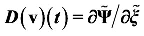
) . Let us define also the dimensionless acceleration-deceleration function for the quasi-stationary regime
 , (52)
as an analogue of the dimensionless deceleration function  which was used in [28].
One obtains for the approximation (31) and SYSTEM 2:
 ,
,  ,
,  ,
,  ,
,  ,
,  ,
,  ,
, .
.
Figures 17 and 18 correspond to G = 1. From these calculations follow:
1) As it was waiting the quasi-stationary regime exists only in the restricted (on the left and on the right sides) area. Out of these boundaries the explicit time dependent regime should be considered. But it is not the Hubble regime.
2) In the Hubble regime one obtains the negative area (low part of the dash-dotted curve of Figure 17). It corresponds to the self-consistent force acting along the expansion of the local flow.
3) The dependence of  is not linear (see Figure 18), more over the curvature contains maximum. The area of acceleration placed between two areas of the deceleration.
Let us show now the result of calculations for another  approximation in the simplest possible form, namely (see also (33))
 . One obtains for this
  - approximation and SYSTEM 2 for G = 1, see Figures 19-22.
We can add to the previous conclusions:
4) Approximation  conserves all principal characters of the previous dependences, but the area of the Hubble regime becomes larger.
5) Approximation  allows realizing the
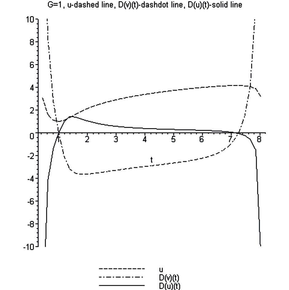
Figure 17. Dependence of the acceleration-deceleration function  (in Maple notation
 ), derivation of the self-consistent potential
  and velocity
  on the radial distance
 .
.
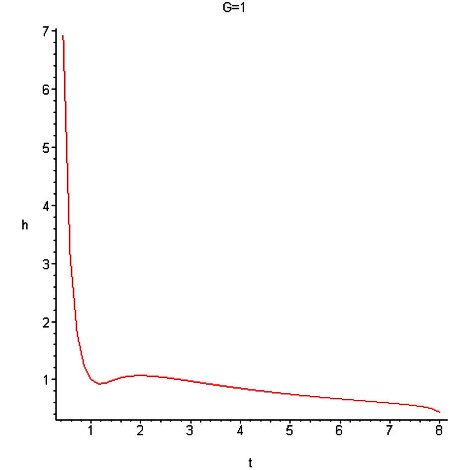
Figure 18. Dependence of the dimensionless Hubble parameter on the radial distance.
numerical transition to the “classical” gas dynamics of explosions. By the  there are no Hubble regimes in principal.
6) Diminishing of G leads to diminishing of the area of the Hubble regime with the positive acceleration of the matter catched by the self-consistent gravitational field.
7) Dependence of  does not contain the maxi-
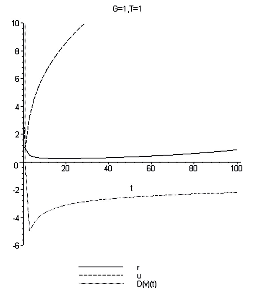
Figure 19. r density , u
, u ,
, .
.
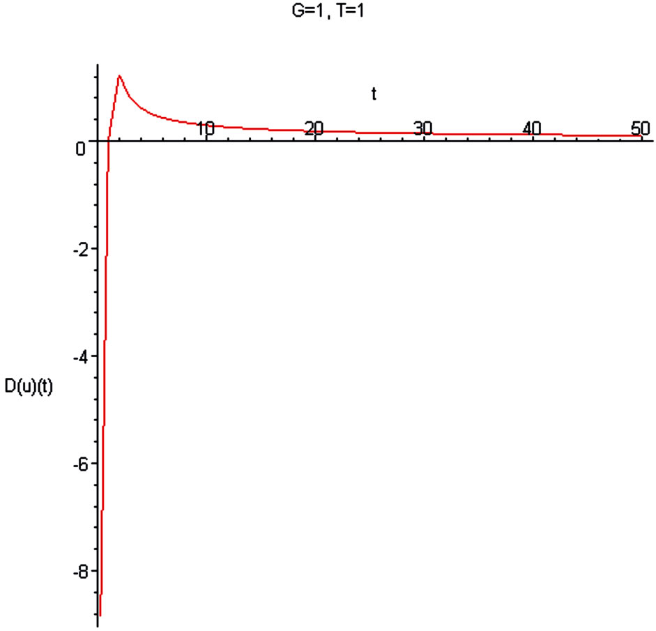
Figure 20. Dependence of the acceleration-deceleration  on
on .
.
mum on the curve for the small value of parameter G (Aregime). It is reasonable to find from the observation the Hubble boxes where A-regime is realizing. Consideration of the Local Group evolution of galaxies (see Figure 16) leaves the impression that this burst responds to the PRS-regime.
As we see the Hubble expansion with acceleration is explained as result of mathematical modeling based on the principles of non-local physics. Peculiar features of
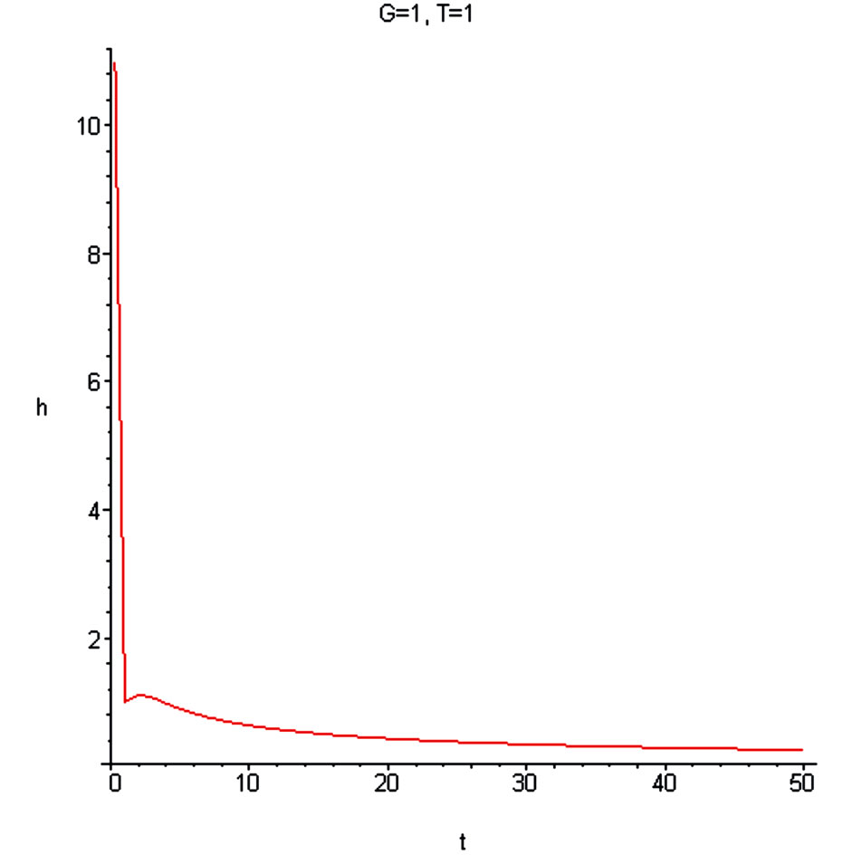
Figure 21. Dependence of the dimensionless Hubble parameter on the radial distance for G = 1.
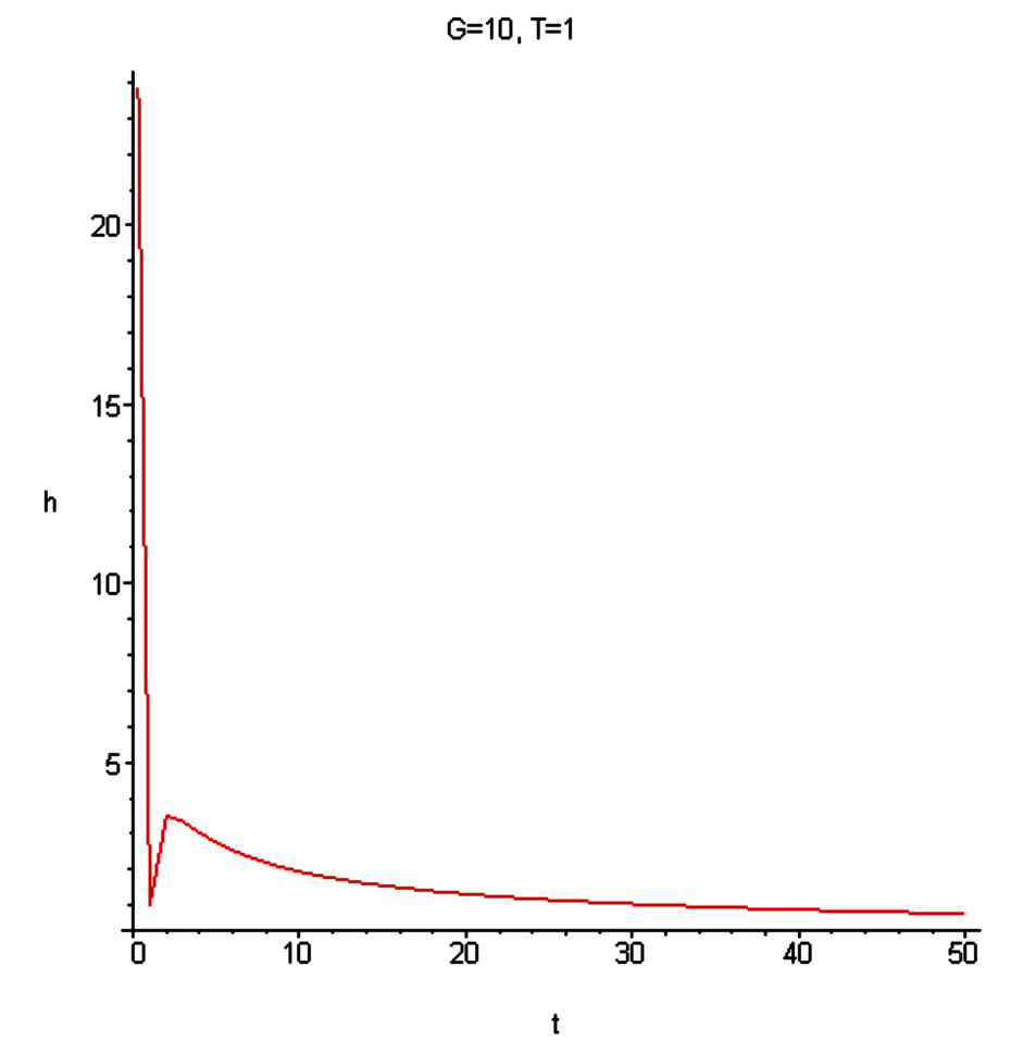
Figure 22. Dependence of the dimensionless hubble parameter on the radial distance for G = 10.
the rotational speeds of galaxies and the Hubble expansion with acceleration need not in the introduction of new essence like dark matter and dark energy.
4. Conclusion
The unified generalized non-local theory is applied for mathematical modeling of cosmic objects with success. For the case of galaxies the theory leads to the flat rotation curves known from observations. The transformation of Kepler’s regime into the flat rotation curves for different solitons is shown. The origin of Hubble effect (including the matter expansion with acceleration) is selfcatching of the expanding matter by the self-consistent gravitational field in conditions of weak influence of the central massive bodies. The Hubble expansion with acceleration is obtained as result of mathematical modeling based on the principles of non-local physics. Peculiar features of the rotational speeds of galaxies and effects of the Hubble expansion need not in the introduction of new essence like dark matter and dark energy. The origin of difficulties consists in the total Oversimplification following from the principles of local physics.
REFERENCES
- V. Rubin and W. K. Ford Jr., “Rotation of the Andromeda Nebula from a Spectroscopic Survey of Emission Regions,” Astrophysical Journal, Vol. 159, 1970, p. 379. Hdoi:10.1086/150317
- V. Rubin, N. Thonnard and W. K. Ford Jr., “Rotational Properties of 21 Sc Galaxies with a Large Range of Luminosities and Radii from NGC 4605 (R = 4 kpc) to UGC 2885 (R = 122 kpc),” Astrophysical Journal, Vol. 238, 1980, pp. 471-487. Hdoi:10.1086/158003
- M. Milgrom, “The MOND Paradigm,” ArXiv Preprint, 2007. http://arxiv.org/abs/0801.3133v2
- A. D. Chernin, “Dark Energy and Universal Antigravitation,” Physics-Uspekhi, Vol. 51, No. 3, 2008, pp. 267-300. Hdoi:10.1070/PU2008v051n03ABEH006320
- J. S. Bell, “On the Einstein Podolsky Rosen Paradox,” Physics, No. 1, 1964, pp. 195-200.
- B. V. Alexeev, “Generalized Boltzmann Physical Kinetics,” Elsevier, Amsterdam, 2004.
- L. Boltzmann. “Weitere Studien über das Warmegleichgewicht unter Gasmoleculen,” Sitzungsberichte der Kaiserlichen Akademie der Wissenschaften, Vol. 66, 1872, p. 275.
- L. Boltzmann, “Vorlesungen über Gastheorie,” Verlag von Johann Barth, Zweiter Unveränderten Abdruck. 2 Teile, Leipzig, 1912.
- N. N. Bogolyubov, “Problemy Dinamicheskoi Teorii v Statisticheskoi Fizike, (Dynamic Theory Problems in Statistical Physics),” Moscow Leningrad Gostekhizdat, 1946.
- M. Born and H. S. Green. “A General Kinetic Theory of Liquids,” Proceedings of the Royal Society, Vol. 188, No. 1012, 1946, pp. 10-18. Hdoi:10.1098/rspa.1946.0093
- H. S. Green, “The Molecular Theory of Fluids,” NorthHolland, Amsterdam, 1952.
- J. G. Kirkwood, “The Statistical Mechanical Theory of Transport Processes 2: Transport in Gases,” Journal of Chemical Physics, Vol. 15, No. 1, 1947, pp. 72-76. Hdoi:10.1063/1.1746292
- J. Yvon, “La Theorie Statistique des Fluides et l’Equation d’etat,” Hermann, Paris, 1935.
- B. V. Alekseev, “Matematicheskaya Kinetika Reagiruyushchikh Gazov,” (Mathematical Theory of Reacting Gases), Nauka, Moscow, 1982.
- B. V. Alexeev, “The Generalized Boltzmann Equation, Generalized Hydrodynamic Equations and their Applications,” Philosophical Transactions of the Royal Society of London, Vol. 349, 1994, pp. 417-443. Hdoi:10.1098/rsta.1994.0140
- B. V. Alexeev, “The Generalized Boltzmann Equation,” Physica A, Vol. 216, No. 4, 1995, pp. 459-468. Hdoi:10.1016/0378-4371(95)00044-8
- S. Chapman and T. G. Cowling, “The Mathematical Theory of Non-Uniform Gases,” University Press, Cambridge, 1952.
- I. O. Hirschfelder, Ch. F. Curtiss and R. B. Bird, “Molecular Theory of Gases and Liquids,” John Wiley and sons, Inc., New York, Chapman and Hall, London, 1954.
- Yu. L. Klimontovich, “About Necessity and Possibility of Unified Description of Hydrodynamic Processes,” Theoretical and Mathematical Physics, Vol. 92, No. 2, 1992, p. 312.
- B. V. Alekseev, “Physical Basements of the Generalized Boltzmann Kinetic Theory of Gases,” Physics-Uspekhi, Vol. 43, No. 6, 2000, pp. 601-629. Hdoi:10.1070/PU2000v043n06ABEH000694
- B. V. Alekseev, “Physical Fundamentals of the Generalized Boltzmann Kinetic Theory of Ionized Gases,” Physics-Uspekhi, Vol. 46, No. 2, 2003, pp. 139-167. Hdoi:10.1070/PU2003v046n02ABEH001221
- B. V. Alexeev, “Generalized Quantum Hydrodynamics and Principles of Non-Local Physics,” Journal of Nanoelectronics and Optoelectronics, Vol. 3, No. 2, 2008, pp. 143-158. Hdoi:10.1166/jno.2008.207
- B. V. Alexeev, “Application of Generalized Quantum Hydrodynamics in the Theory of Quantum Soliton Evolution,” Journal of Nanoelectronics and Optoelectronics, Vol. 3, No. 3, 2008, pp. 316-328. Hdoi:10.1166/jno.2008.311
- B. V. Alexeev, “Generalized Theory of Landau Damping,” Journal of Nanoelectronics and Optoelectronics, Vol. 4, No. 1, 2009, pp. 186-199. Hdoi:10.1166/jno.2009.1021
- B. V. Alexeev, “Generalized Theory of Landau Damping in Collisional Media,” Journal of Nanoelectronics and Optoelectronics, Vol. 4, No. 3, 2009, pp. 379-393. Hdoi:10.1166/jno.2009.1054
- S. Perlmutter, et al., “Measurements of Ω and Λ from 42 High-Redshift Supernovae,” Astrophysical Journal, Vol. 517, No. 2, 1999, pp. 565-586. Hdoi:10.1086/307221
- A. G. Riess, et al., “Observational Evidence from Supernovae for an Accelerating Universe and a Cosmological Constant,” Astronomical Journal, Vol. 116, No. 3, 1998, pp. 1009-1038. Hdoi:10.1086/300499
- A. G. Riess, et al., “Type IA Supernova Discoveries at
 from the Hubble Telescope: Evidence for Past Deceleration and Constraints on Dark Energy Evolution,” Astrophysical Journal, Vol. 607, 2004, pp. 665-687. Hdoi:10.1086/383612
 - B. V. Alexeev, “Non-local Physics. Non-Relativistic Theory,” Lambert Academic Press (in Russian), 2011.
- B. V. Alexeev and I. V. Ovchinnikova, “Non-Local Physics. Relativistic Theory,” Lambert Academic Press, 2011, (in Russian).
- B. V. Alexeev, “Application of Non-Local Physics in the Theory of Hubble Expansion,” Nova Science Publishers, Inc., 2011.
- I. D. Karachentsev and O. G. Kashibadze, “Masses of the Local Group and of the M81 Group Estimated from Distortions in the Local Velocity Field,” Astrophysics, Vol. 49, No. 1, 2006, pp. 3-18.
- E. B. Gliner, “The Vacuum-Like State of a Medium and Friedman Cosmology,” Soviet Physics—Doklady, Vol. 15, No. 6, 1970, pp. 559-561.
- L. S. Sparke and J. S. Gallagher III, “Galaxies in the Universe: Introduction,” Cambridge University Press, Cambridge, 2000.