Journal of Modern Physics
Vol.3 No.3(2012), Article ID:18193,4 pages DOI:10.4236/jmp.2012.33030
Relation between the Intervals ΔE and Δt Obtained inthe De-Excitation Process of Electrons in Metals
Institute of Physical Chemistry, Polish Academy of Sciences, Warsaw, Poland
Email: olsz@ichf.edu.pl
Received November 30, 2011; revised January 6, 2012; accepted January 15, 2012
Keywords: De-Excitation of Electrons; Metals; Relations between the Intervals of Energy and Time
ABSTRACT
A relation between the intervals of energy and time, derived in a former paper and associated with the electron transitions on the Fermi surface of a metal, is examined in comparison with the experimental data. These data are obtained from the de-excitation process of electrons in metals. A comparison between theory and experiment demonstrated that the new relation between energy and time is fitted much better for the experimental results than the well-known relation due to the Heisenberg theory.
1. Introduction
A well-known relation between the intervals of energy and time , deduced by Heisenberg [1,2], namely
 (1)
(1)
is often considered as analogous to the uncertainty relation represented by the intervals of the particle position and momentum. However, it has been stressed a time ago that the significance of (1) is entirely different than that of the formula
 (2)
(2)
where  label the coordinates of the position and momentum in a three-dimensional space. In fact (1) concerns the exactly measured intervals of energy and time, whereas (2) refers to the uncertainties of the values of the position and momentum coordinates measured at the same instant of time [3-5]. Nevertheless, the uncertainty relation for energy and time similar to (2) can be also derived [5].
The aim of the present paper is to give a kind of a new look on the relation between  and
and  done from both the theoretical and experimental point of view. In fact the formula in (1) is not a unique proposal of the coupling connecting
  and
and . An alternative formula can be derived when the electron transitions in the electron gas are effectuated in the field of the magnetic induction
 . Let us assume that
  is directed along axis
 , so
, so , and simultaneously the limitations of the electron velocity imposed by the special theory of relativity are also taken into account. In this case a condition satisfied by the change of the momentum square
  at the Fermi surface within the time interval
  becomes [6]:
 (3)
(3)
The momentum change in (3) can be referred to that of energy by multiplying the both sides of (3) by the term
 (4)
(4)
For, this operation gives in place of (3) the relation
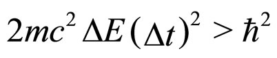 (5)
(5)
if we note the well-known free-electron formula for the change of the Fermi energy:
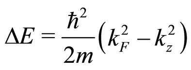 (6)
(6)
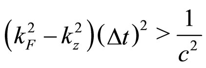
In effect, when instead of (5) the square-root of the both sides of this formula is taken into account, we obtain a different relation between  and
and  than (1):
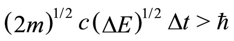 (7)
(7)
A characteristic point is that (7) does not contain , although some limitation for the maximal value of this parameter and, consequently, the cyclotron frequency
  induced in the electron gas, is imposed by the theory [6].
The lack of  makes (7) a competitive expression to (1). Sections 2 and 3 try to clarify this competition on the experimental basis.
2. Experimental Approach
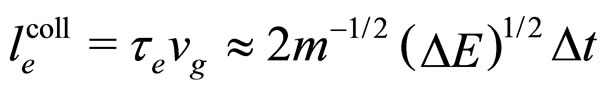
This approach is based on the de-excitaion process of the photoelectrons [7]. In considering the decay of the motion of a photoelectron excited originally from the freeelectron gas we have the notion of the lifetime of that electron in its excited state
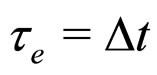 (8)
(8)
and a reference of this lifetime to the electron mean free path
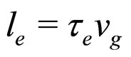 (9)
(9)
 is the group velocity of a photoelectron in its excited state.
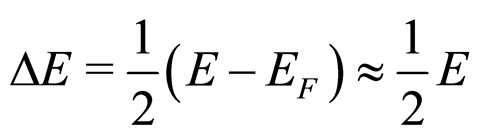
The amount of energy lost by the excited electron of energy  in the de-excitation process is most often in the range of magnitude
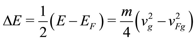 (10)
(10)
 is the group velocity of an electron on the Fermi level. The relation in (10) holds because, due to the interaction of an excited electron with a less energetic electron, the photon energy is shared between two excited electrons [7].
In case a collective motion of the conduction electrons is taken into account, the plasmon scattering from the interaction of the excited electron with a set of conduction electrons should be considered. In this circumstanc  in (9) is modified into
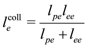 (11)
(11)
Here  is coming from the plasmon scattering and
  from the electron-electron scattering [7].
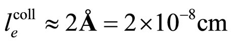
A characteristic experimental result [7,8] is that for large  the length
  which replaces
  in (9) tends approximately to a constant value independent of
 . This result substituted to (9) provides us with the relation
 (12)
(12)
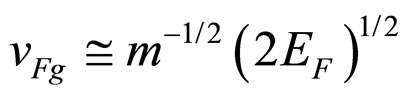
Another relation for the excited electron is its group velocity
 (13)
(13)
because of the well-known formula for the kinetic energy. At the end of the de-excitation process the electron is close to the Fermi level, so its velocity is decreased to
 (14)
(14)
In many excited cases, for example in the Auger effect where  of few hundreds of eV are involved, we have
 (15)
(15)
because  is so small that it can be approximately neglected in comparison with large
 . For example, in the metallic Cs examined in the photoexcitation process,
  is smaller than 1.6 eV [9]. Consequently, due to (8), (13) and (15):
 (16)
(16)
because  in (13) is approximately equal to
 .
.
A characteristic point is that the result obtained in (16) differs from the expression on the left-hand side of (7) only by a constant factor. In effect, because  is a constant and
 , the relation (16) between
  and
and —considered with the accuracy to a constant coefficient—becomes much similar to that obtained in (7). By applying (16) in (7) we obtain the formula
 (17)
(17)
A numerical check of validity of this relation is done in Section 3.
3. Discussion
The experimental result obtained for  in (16) is as follows [7,8]:
 (18)
(18)
The value can be subsequently substituted into (17). In view of the fundamental constants of nature used in the calculations we obtain
 (19)
(19)
which implies that relation (17) is satisfied, at least in the examined case.
Considering the relations between energy and time, there is, however, nothing special in the photoexcitation of a metal electron. Another well-known excitation can be, for instance, due to external electric field effect on the electrons. For very pure metals, the effect offers another mean free path of the electron than that considered in (17). This path, which is characteristic for the conduction process in a given metal, is due to electron interaction with the phonon medium combined with the medium of other electrons. The path length labelled by , is an equilibrium parameter for electron transport in the electric field, virtually independent of the field strength. As a result, instead of (17), we arrive at the formula:
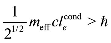 (20)
(20)
Here  is the effective electron mass in the conductivity process.
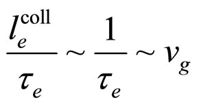
As the tansport involves mainly the electrons close to the Fermi level, we have
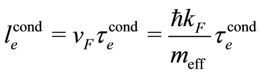 (21)
(21)
where  is the relaxation time characteristic for conduction. The formula (21) transforms (20) into
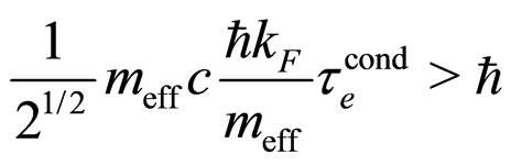 (22)
(22)
equivalent to a simple relation
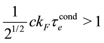 (23)
(23)
For  cm/s,
cm/s,  and
and 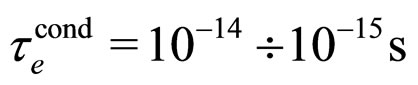 at room temperature, as valid for most metals [9], the relation (23) is obviously satisfied by the experimental data.
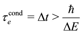
A separate estimate of  alone can be done on the basis of (3). This parameter is also assumed to approximate the decay time of the excited electron:
 (24)
(24)
For  close to
  we can put
 (25)
(25)
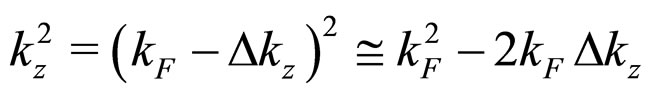
where  is considered to be a small fraction of the Bloch vector component
 :
:
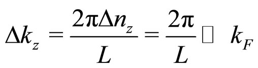 (26)
(26)
we have put  and
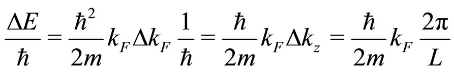
and  is the edge length of a cubic metal volume. As a result, the relation (3) becomes
 (27)
(27)
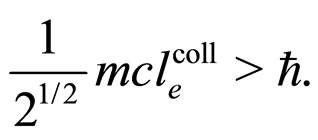
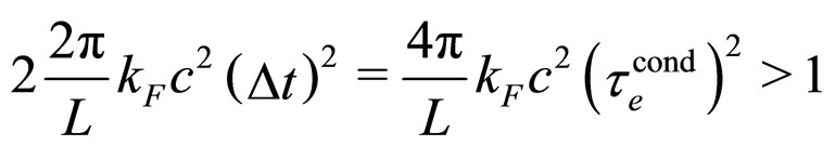
Therefore, we should have:
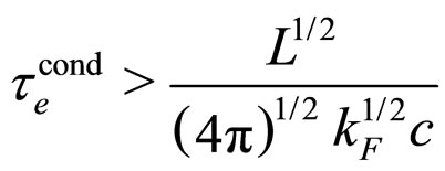 (28)
(28)
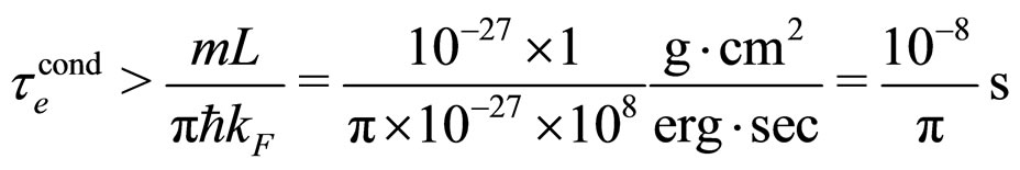
For  cm and
 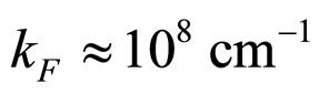 we obtain from (28) the condition
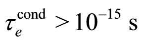 (29)
(29)
which is a number approaching rather perfectly the experimental value  for metals [9].
Let us note that the formula (1) which is in competition with (7) gives
 (1a)
(1a)
Here
 (28a)
(28a)
on condition the equality 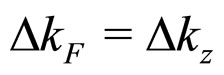 is applied for
  calculated in (26). A substitution of (28a) into (1a) gives
 (29a)
(29a)
This result exceeds by many orders a typical experimental  in metals measured at normal conditions characterized by the room temperature; see [9] and (29).
A comparison of the Heisenberg relation (1) with the present one in (7) can be done also by considering an individual electron excitation due to the electric field effect. In this case from (1) and the experimental  put for
  we have
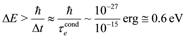 (30)
(30)
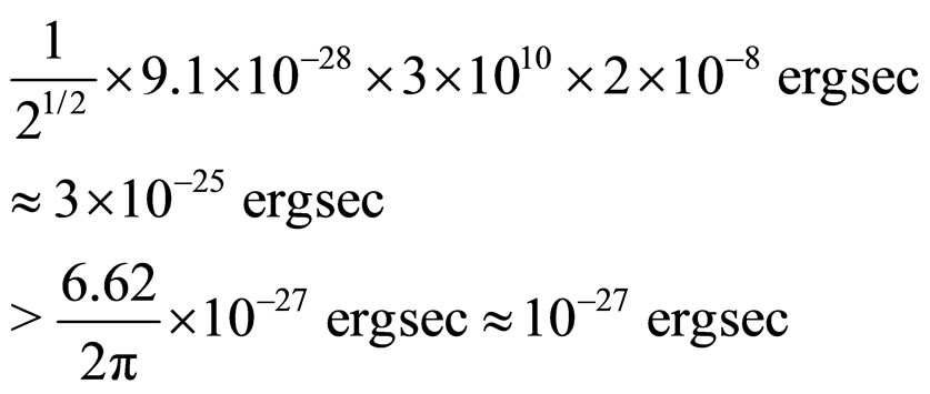
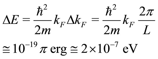
which is an unrealistically high energy. On the other hand, formula (7) gives:
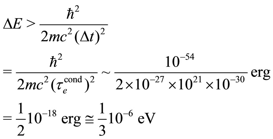 (31)
(31)
which is a much more reasonable value for an elementary excitation energy of an electron in the conduction process. In fact, a low excitation energy at the Fermi level is that entering (28a):
 (32)
(32)
This is close to the result in (31).
4. Conclusions
The experimental results obtained for parameters related to the de-excitation of electrons in metals seem to favourite much more the relation (7) between  and
and  than the relation given in (1). A problem may arise, however, as to what extent the formula (7) can be useful in the case of non-free-electron transitions.
Another point concerns an agreement between (31) and (32). A so good agreement is probably an accidental since  is a parameter strongly dependent on the temperature
 , especially at low
 . For T nearly 273 K, as usually used in the presentation of the experimental data, the dependence of
  on
on  is rather weak. Consequently, the same dependence should apply to the mean free-electron path which tends to become an approximately constant parameter, in agreement with the behaviour of
  discussed in Section 2.
REFERENCES
- W. Heisenberg, “Ueber den Anschaulichen Inhalt der Quantentheoretischen Kinematik und Mechanik,” Zeitschrift fuer Physik, Vol. 43, No. 3-4, 1927, pp. 172-198. doi:10.1007/BF01397280
- L. I. Schiff, “Quantum Mechanics,” 3rd Edition, McGrawHill, New York, 1968.
- L. D. Landau and E. M. Lifshitz, “Quantum Mechanics,” Pergamon, Oxford, 1965.
- M. Jammer, “The Philosophy of Quantum Mechanics,” Wiley, New York, 1974.
- W. Schommers, “Space-Time and Quantum Phenomena,” In: W. Schommers, Ed., Quantum Theory and Pictures of Reality, Springer, Berlin, 1989, pp. 217-277.
- S. Olszewski, “Magnetic Field Induction and Time Intervals of the Electron Transitions Approached on a Classical and Quantum-Mechanical Way,” Journal of Modern Physics, Vol. 2, No. 11, 2011, pp. 1305-1309. doi:10.4236/jmp.2011.211161
- P. J. Vernier, “Photoemission,” In: E. Wolf, Ed., Progress in Optics, Vol. 14, North-Holland, Amsterdam, 1976, pp. 245-325.
- N. V. Smith and G. B. Fischer, “Photoemission Studies of the Alkali Metals. II. Rubidium and Caesium,” Physical Review B, Vol. 3, No. 11, 1971, pp. 3662-3670. doi:10.1103/PhysRevB.3.3662
- N. W. Ashcroft and N. D. Mermin, “Solid State Physics,” Holt, Rinehart and Winston, New York, 1976.