Applied Mathematics
Vol.08 No.04(2017), Article ID:75530,16 pages
10.4236/am.2017.84035
Boundedness of Calderón-Zygmund Operator and Their Commutator on Herz Spaces with Variable Exponent
Omer Abdalrhman1,2*, Afif Abdalmonem1,3, Shuangping Tao1
1College of Mathematics and Statistics, Northwest Normal University, Lanzhou, China
2College of Education, Shendi University, Shendi, River Nile State, Sudan
3Faculty of Science, University of Dalanj, Dalanj, South kordofan, Sudan

Copyright © 2017 by authors and Scientific Research Publishing Inc.
This work is licensed under the Creative Commons Attribution International License (CC BY 4.0).
http://creativecommons.org/licenses/by/4.0/


Received: March 13, 2017; Accepted: April 17, 2017; Published: April 20, 2017
ABSTRACT
The aim of this paper is to study the boundedness of Calderón-Zygmund operator and their commutator on Herz Spaces with two variable exponents
. By applying the properties of the Lebesgue spaces with variable exponent, the boundedness of the Calderón-Zygmund operator and the commutator generated by BMO function and Calderón-Zygmund operator is obtained on Herz space.
Keywords:
Calderón-Zygmund Operator, Commutator, Herz Spaces with Variable Exponent, BMO Spaces

1. Introduction
Definition 1.1. Let
be a bounded linear operator from
to
(see [1] , [2] ).
is called a standard operator if
satisfies the following conditions:
1)
extends to a bounded linear operator on
.
2) There exists a function
defined by
satisfies
(1.1)
where
.
3)
for
with
A standard operator
is called a
-Calderón
Zygmund operator if
is a standard kernel satisfies:
(1.2)
(1.3)
if
for some
.
The bounded mean oscillation BMO space and BMO norm are defined, respectively, by
(1.4)
(1.5)
The commutator of the Calderón-Zygmund operator is defined by
(1.6)
In 1983, J.-L. Jouné proved
-Calderón
Zygmund operator is bounded on
in [3] . Coifman, Rochberg and Weiss proved that commutator [b,T] is bounded on
(see [4] ).
Kovácik and Rákosník introduced Lebesgue spaces and Sobolev spaces with variable exponents (see [5] ). The function spaces with variable exponent has been recently obtained an increasing interest by a number of authors since many applications are found in many different fields, for example, in fluid dynamics (see [6] ), image restoration (see [7] [8] [9] ) and differential equations.
Herz spaces play an important role in harmonic analysis. After they were introduced in [10] , the boundedness of some operators and some characteriza- tions of Herz spaces with variable exponents were studied extensively (see [11] - [16] ). In 2015, Wang and Tao introduced the Herz spaces with two variable exponents
, and studied the parameterized Littlewood-Paley operators and their commutators on Herz spaces with variable exponents in [17] .
In this paper, we will discuss the boundedness of the Calderón-Zygmund operator
and their commutator
are bounded on Herz spaces with two variable exponents
.
2. Definitions of Function Spaces with Variable Exponent
In this section we recall some definitions. Let
be a measurable set in
with
. We firstly recall the definition of the Lebesgue spaces with variable exponent.
Definition 2.1. [5] Let
be a measurable function. The Lebesgue space with variable exponent
is defined by
(2.1)
For all compact
, the space
is defined by
(2.2)
The Lebesgue spaces
is a Banach spaces with the norm defined by
(2.3)
We denote
. Then
consists of all
satisfying
and
. Let
be the Hardy-Littlewood maximal operator. We denote
to be the set of all function
satisfying the
is bounded on
.
Definition 2.2. [18] Let
. The mixed Lebesgue sequence space with variable exponent
is the collection of all sequences
of the measurable functions on
such that
(2.4)
Let
,
, for
, we have that
(2.5)
Let
,
Definition 2.3. [17] Let
. The homogeneous Herz space with variable exponent
is defined by
Equipped the norm
Remark 2.1. [17] Let
satisfying
and satisfy the following results:
1)
2) If
and
. For any
, by using Lemma 3.7 and Remark 2.2, we have
where
This implies that
.
Remark 2.2. Let
. Then we have
where
3. Properties and Lemmas of Variable Exponent
In this section, we recall some properties and some lemmas of variable exponent belonging to the class
.
Proposition 3.1. [19] If
satisfies
(3.1)
(3.2)
Hence we have
.
Lemma 3.1. [5] Given
have that for all functions
and
,
(3.3)
where
.
Lemma 3.2. [5] Suppose that
, for any
, when
, we get
(3.4)
where
.
Proposition 3.2. [20] Let
and
be a Calderón
Zygmund operator. Then we have
(3.5)
Lemma 3.3. [20] Let
function and
be a Calderón
Zygmund operator.Then
(3.6)
Lemma 3.4. [11] Let
. If
with
, then we have
1.
2.
Lemma 3.5. [21] Let
, then there exist constants
, and
such that for all balls
and all measurable subset
,
(3.7)
Lemma 3.6. [11] If
, there exist a constant
such that for any balls B in
, we have
(3.8)
Lemma 3.7. [17] Suppose that
. If
, then
(3.9)
4. The Main Theorems and Their Proofs
Theorem 4.1. Suppose that
with
. If
with
as defined in Lemma 3.5, then the operator
is bounded from
to
.
Proof Let
. We write
By Definition 2.3, we have
#Math_135# (4.1)
Since
(4.2)
where
(4.3)
(4.4)
and
Thus,
We easily see that
(4.6)
This implies that we only need to prove
. Denote
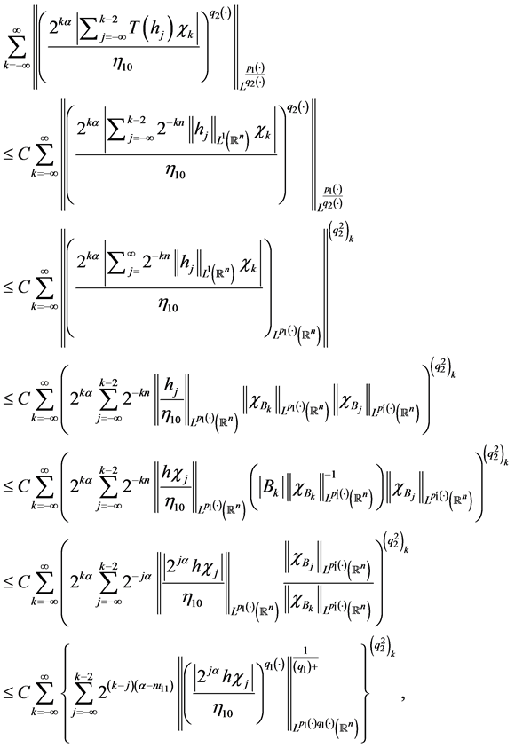
First, we consider
. By virtue of Lemma 3.7, we get
(4.7)
where,
In the above, we use the Proposition 3.2 and Remark 2.2. Since
, we have
and
, we get
Here
and
. That is
(4.8)
Let us now turn to estimate
. Noting that
and
, by the generalized Hölder's inequality and the Minkowski’s inequality, we get
(4.9)
By Lemmas 3.5-3.7 and the fact that
, we easily see that
 (4.10)
where
Therefore, if
and
, we can get
where
.
If
and
. By Remark 2.2 and applying the generalized Hölder’s inequality, we obtain
where
.
Hence, we see that
(4.11)
Finally, we estimate
. Noting that for each
and
, we have
(4.12)
By Lemma 3.7 and
, we get
 (4.13)
where
Then we have
, by using the same argument in
. Thus, we prove Theorem 4.1.
Theorem 4.2. Let
. Suppose that
with
. If
with
as defined in lemma 3.5, then the commutator
is bounded from
to
.
Proof Let
.We write
By virtue of the definition of
, we have
(4.14)
Since
(4.15)
Let
(4.16)
(4.17)
(4.18)
and
Therefore, we can obtain
Thus it follows that,
(4.20)
Hence
. Denoting
, firstly we estimate
as in Theorem 4.1. Applying Lemma 3.3, we imme- diately arrive at
So we can get that
(4.21)
Next we estimate
, Let
.
(4.22)
Thus, from Lemmas 3.4-3.7, We obtain that
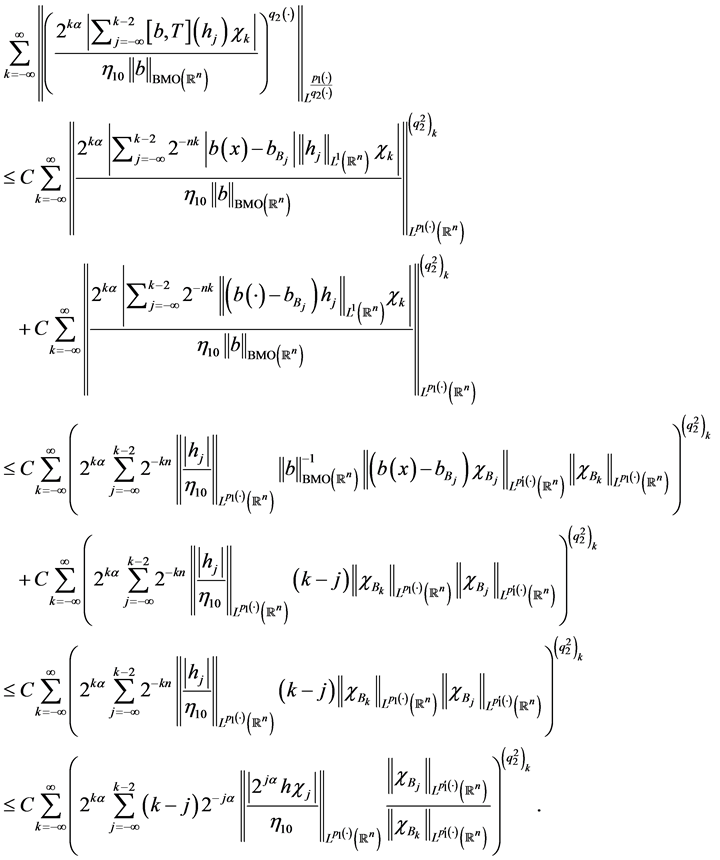
Therefore, we get
(4.23)
where
This, for
,
, along with Remark 2.2, tells us that
where
If
, it is follows from Remark 2.2 and Hölder’s inequality that
where
.
This implies that
(4.24)
Finally we estimate
, for any
, by the same way to argument in
, we obtain that
(4.25)
and
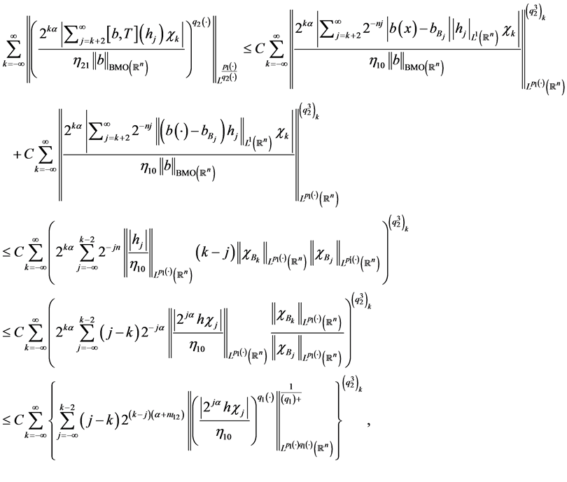 (4.26)
where
Hence, we arrive at that
by the similar argument in the proof Theorem 4.1.
This completes the proof of Theorem 4.2.
Acknowledgements
This paper is supported by National Natural Foundation of China (Grant No. 11561062).
Cite this paper
Abdalrhman, O., Abdalmonem, A. and Tao, S.P. (2017) Boundedness of Calderón-Zygmund Operator and Their Commutator on Herz Spaces with Variable Exponent. Applied Mathematics, 8, 428-443. https://doi.org/10.4236/am.2017.84035
References
- 1. Calderón, A. and Zygmund, A. (1956) On Singular Integrals. American Journal of Mathematics, 78, 289-309. https://doi.org/10.2307/2372517
- 2. Calderón, A. and Zygmund, A. (1978) On Singular Integral with Variable Kernels. Applied Analysis, 7, 221-238. https://doi.org/10.1080/00036817808839193
- 3. Jouné, J.-L. (1983) Calderón-Zygmund Operators, Pseudo-Differential Operators and the Cauchy Integral of Calderón. In: Lecture Notes in Math, Vol. 994, Springer-Verlag, Berlin, Heidelberg.
- 4. Coifman, R., Rochberg, R. and Weiss, G. (1976) Factorization Theorems for Hardy Spaces in Several Variables. Annals of Mathematics, 103, 611-635.
https://doi.org/10.2307/1970954
- 5. Kovácik, O. and Rákosník, J. (1991) On Spaces Lp(x) and Wk,p(x). Czechoslovak Mathematical Journal, 41, 592-618.
- 6. Diening, L. and Ruicka, M. (2003) Calderón-Zygmund Operators on Generalized Lebesgue Spaces Lp(.) and Problems Related to Fluid Dynamics. Journal für die Reine und Angewandte Mathematik, 563, 197-220.
https://doi.org/10.1515/crll.2003.081
- 7. Chen, Y., Levine, S. and Rao, M. (2006) Variable Exponent, Linear Growth Functionals in Image Restoration. SIAM Journal on Applied Mathematics, 66, 1383-1406. https://doi.org/10.1137/050624522
- 8. Li, F., Li, Z. and Pi, L. (2010) Variable Exponent Functionals in Image Restoration. Applied Mathematics and Computation, 216, 870-882.
- 9. Harjulehto, P., Hasto, P., Latvala, V. and Toivanen, O. (2013) Critical Variable Exponent Functionals in Image Restoration. Applied Mathematics Letters, 26, 56-60.
- 10. Izuki, M. (2009) Herz and Amalgam Spaces with Variable Exponent, the Haar Wavelets and Greediness of the Wavelet System. East Journal on Approximations, 15, 87-109.
- 11. Izuki, M. (2010) Boundedness of Commutators on Herz Spaces with Variable Exponent. Rendiconti del Circolo Matematico di Palermo, 59, 199-213.
https://doi.org/10.1007/s12215-010-0015-1
- 12. Izuki, M. (2010) Fractional Integrals on Herz-Morrey Spaces with Variable Exponent. Hiroshima Mathematical Journal, 40, 343-355.
- 13. Wang, L. and Tao, S. (2014) Boundedness of Littlewood-Paley Operators and Their Commutators on Herz-Morrey Spaces with Variable Exponent. Journal of Inequalities and Applications, 2014, 227. https://doi.org/10.1186/1029-242x-2014-227
- 14. Wang, L. and Tao, S. (2015) Parameterized Littlewood-Paley Operators and Their Commutators on Lebegue Spaces with Variable Exponent. Analysis in Theory and Applications, 31, 13-24.
- 15. Tan, J. and Liu, Z. (2015) Some Boundedness of Homogeneous Fractional Integrals on Variable Exponent Function Spaces. ACTA Mathematics Science (Chinese Series), 58, 310-320.
- 16. Omer, A., Afif, A. and Tao, S. (2016) The Boundedness for Commutators of Calderón-Zygmund Operator on Herz-Tybe Hardy Spaces with Variable Exponent. Journal of Applied Mathematics and Physics, 4, 1157-1167.
https://doi.org/10.4236/jamp.2016.46120
- 17. Wang, L. and Tao, S. (2016) Parameterized Littlewood-Paley Operators and Their Commutators on Herz Spaces with Variable Exponents. Turkish Journal of Mathematics, 40, 122-145. https://doi.org/10.3906/mat-1412-52
- 18. Cuz-Uribe, D., Fiorenza, A., Martell, J.M. and Perez, C. (2006) The Boundedness of Classical Operators on Variable Lp Spaces. Annales Academiae Scientiarum Fennicae-Mathematica, 31, 239-264.
- 19. Almeida, A., Hasanov, J. and Samko, S. (2008) Maximal and Potential Operators in Variable Exponent Morrey Spaces. Georgian Mathematical Journal, 15, 195-208.
- 20. Cruz-Uribe, D. and Fiorenza, A. (2013) Variable Lebesgue Spaces: Foundations and Harmonic Analysis. In: Applied and Numerical Harmonic Analysis, Springer, New York.
- 21. Diening, L. (2005) Maximal Function on Musielak-Orlicz Spaces and Generalized Lebesgue Spaces. Bulletin des Sciences Mathématiques, 129, 657-700.
https://doi.org/10.1016/j.bulsci.2003.10.003


 (4.26)