Applied Mathematics
Vol.4 No.11C(2013), Article ID:38300,6 pages DOI:10.4236/am.2013.411A3002
Approximation by Splines of Hermite Type
Faculty of Mathematics and Mechanics, St. Petersburg State University, St. Petersburg, Russia
Email: Yuri.Demjanovich@gmail.com, burovaig@mail.ru
Copyright © 2013 Yuri K. Dem’yanovich, Irina G. Burova. This is an open access article distributed under the Creative Commons Attribution License, which permits unrestricted use, distribution, and reproduction in any medium, provided the original work is properly cited.
Received July 24, 2013; revised August 24, 2013; accepted August 31, 2013
Keywords: Splines; Errors of Approximations
ABSTRACT
The approximation evaluations by polynomial splines are well-known. They are obtained by the similarity principle; in the case of non-polynomial splines the implementation of this principle is difficult. Another method for obtaining of the evaluations was discussed earlier (see [1]) in the case of nonpolynomial splines of Lagrange type. The aim of this paper is to obtain the evaluations of approximation by non-polynomial splines of Hermite type. Considering a linearly independent system of column-vectors ,
, . Let
. Let  be square matrix. Supposing that
  and
and  are columns with components from the linear space
  such that
 . Let
. Let  be vector with components
  belonging to conjugate space
 . For an element
  we consider a linear combination of elements
 :
:  By definition, put
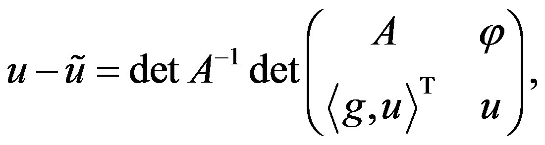
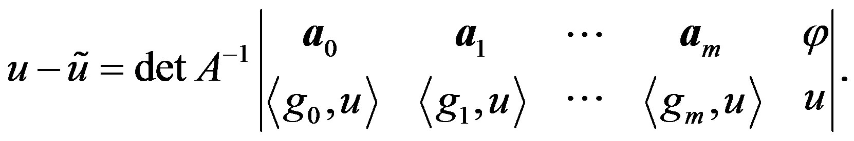
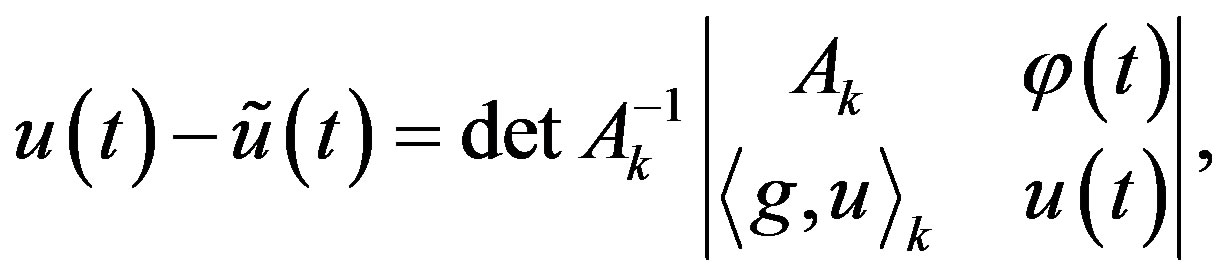
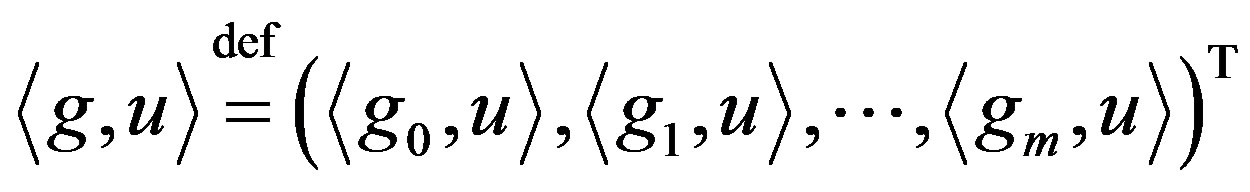 . The discussions are based on the next assertion. The following relation holds:
  where the second factor on the right-hand side is the determinant of a block-matrix of order m + 2. Using this assertion, we get the representation of residual of approximation by minimal splines of Hermite type. Taking into account the representation, we get evaluations of the residual and calculate relevant constants. As a result the obtained evaluations are exact ones for components of generated vector-function
 .
.
1. Representation of Approximation Residual
For convenience we shall give scheme of representation of the approximation residual in general situation (see also [1]).
We consider a linearly independent system of columnvectors  (where m is a natural number)
in the space . The matrix
  composed of these columns is denoted by
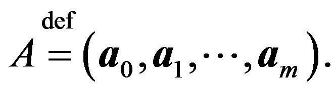 (1)
(1)
Let  be linear space.
Suppose that  and
and
 are columns with components belonging to the space
 ; assume the relation
 (2)
(2)
is valid; matrix A is defined by (1).
Let  be vector with components
 belonging to conjugate space
 .
.
For an element  we consider a linear combination of elements
 :
:
 (3)
(3)
From (2) and (3) it follows that
 (4)
(4)
where  denotes the column-vector in
 namely,
 . The outer round brackets in (4) mean the inner product of
  -dimensional vectors.
Theorem 1 The following relation holds:
 (5)
(5)
where the second factor on the right-hand side is the determinant of a block-matrix of order .
.
Proof By (4), we have  Hence
Hence
 (6)
(6)
where  is the cofactor of an entry
  of the matrix
 . By (6), we can represent the difference
  as the product of determinants, written as
 (7)
(7)
The equality (7) is equivalent to the equality (5).
2. Representation of the Remainder of Approximation by Elementary Hermite Type Splines
On  we consider a grid of the form
We set
Let  be
be  -component vector-function with components in
 . We assume that Wronskian of the components is separated from zero.
Consider function ,
,  , and introduce notation
 (8)
(8)
Let symbol  denote the number of elements of a set
 .
.
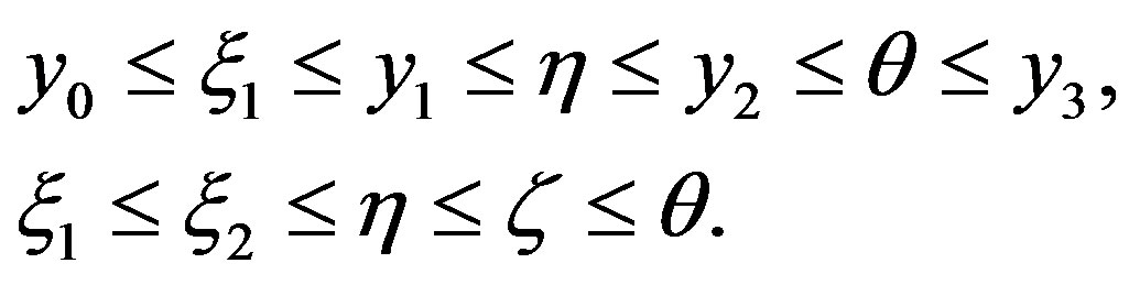
We assume that natural numbers  comply with relations
 ,
,  ,
,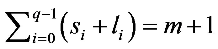 .
.
By definition, put
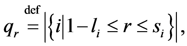
where . Obviously
 .
.
We introduce the functions  by the approximate relations
 (9)
(9)

Consider square matrix  of the order
  (see notation (8)),
and vector-function
then the relations (9) may be rewritten as
It can be proved (for example, see [2]) that the matrix  is invertible. Hence the functions
  are defined uniquely and they are linear independent. If
 ,
,  , then the functions
  belong to
 , and functional system
  defined by formula
is biorthogonal to the system  so that

Rewrite the system (9) in the form
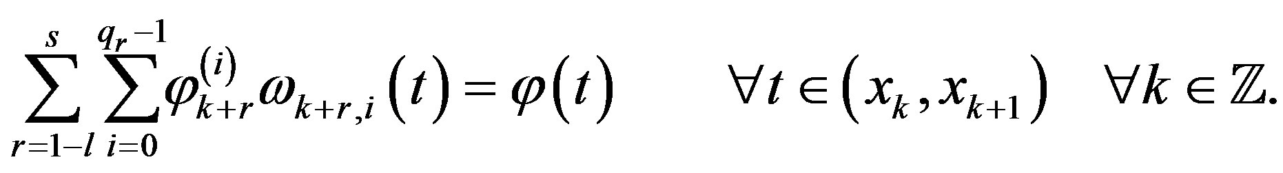 (10)
(10)
Under condition  we have

Analogously on the adjacent interval we get

Discuss the linear space
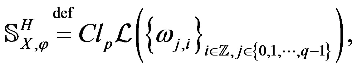
where  is the linear hull of the elements in the curly brackets and
  means the closure of the linear hull in the topology of pointwise convergence.
We call  the space of elementary Hermite type
  -splines.
By definition, put
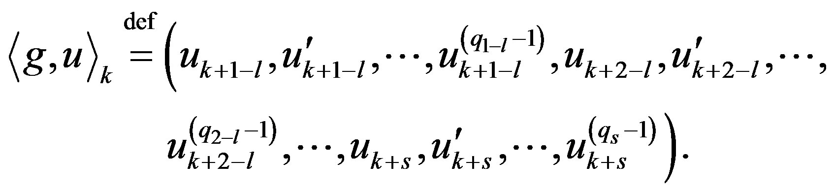
We consider the function  defined by
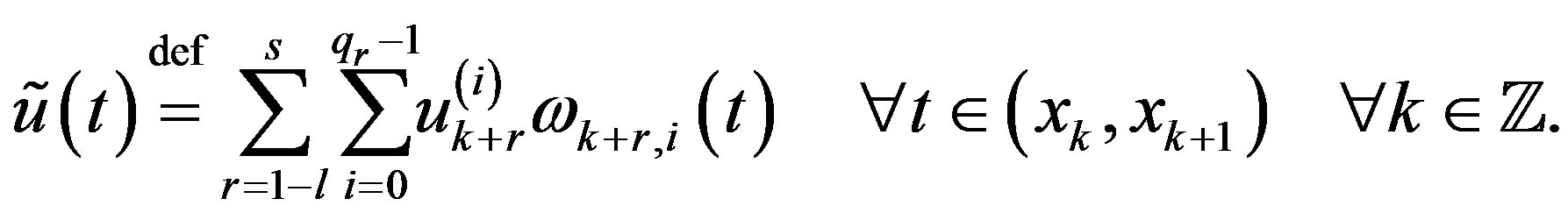 (11)
(11)
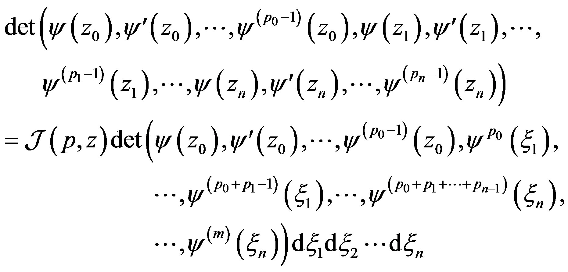
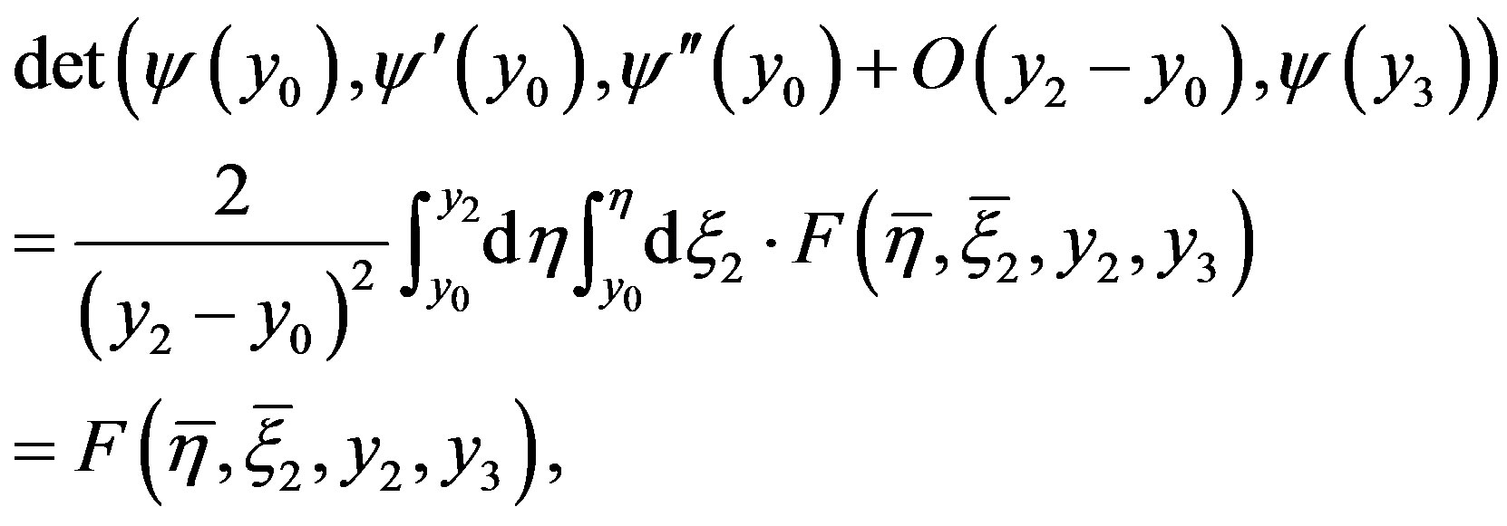
Theorem 2 For ,
,  ,
,
 (12)
(12)
where the second factor on the right-hand side is the determinant of the square matrix of order  written in the block form.
Proof We can obtain the identity (12) by expanding the second determinant of right part of (12) and by usage of the relations (10)-(11) (cf. [1]).
3. Some Auxiliary Assertions
Let ,
,  be natural numbers with property
 ; let
; let  be real numbers, which comply with inequalities
  . Let us put
 ,
, .
.
Lemma 1 For arbitrary  -component vector-function
  the representation
 (13)
(13)
is valid; here  is a linear operator of integration over parallelepiped
with nonnegative kernel.
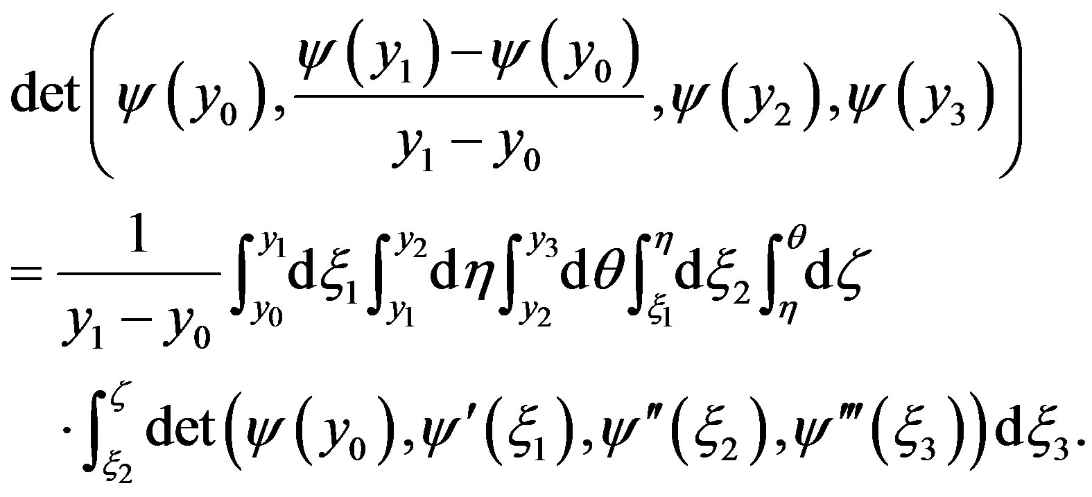
Proof We consider the case 
 ,
, . Introduce value
  with property
  and use notation
 (14)
(14)
so that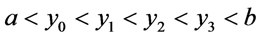 .
.
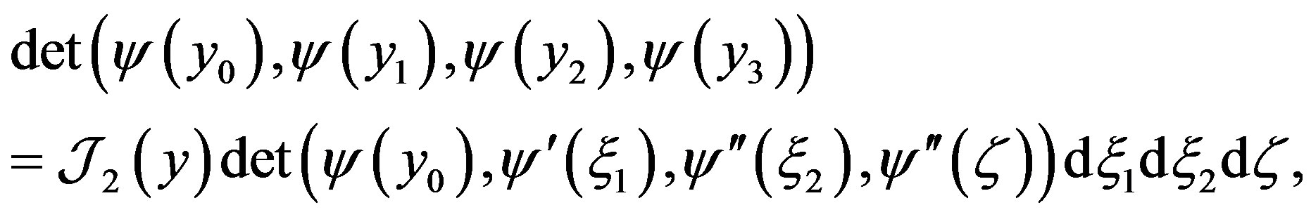
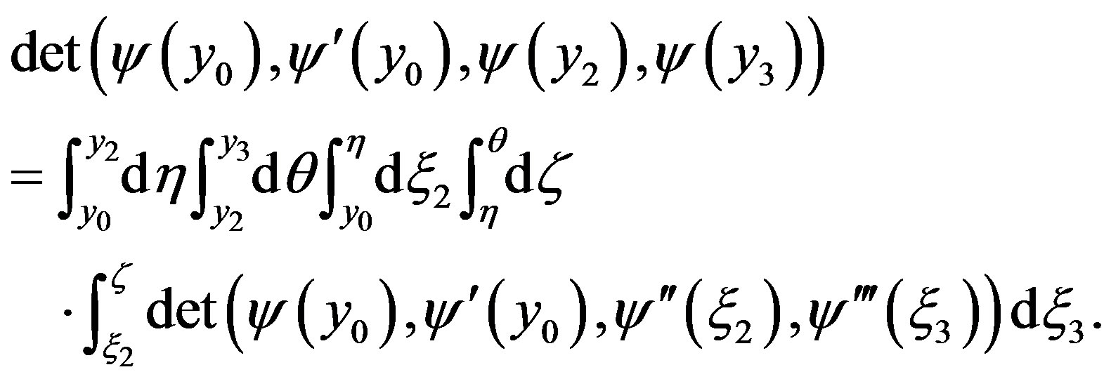
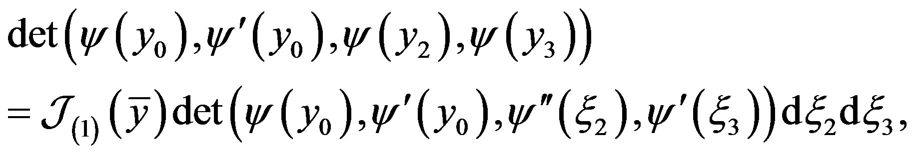
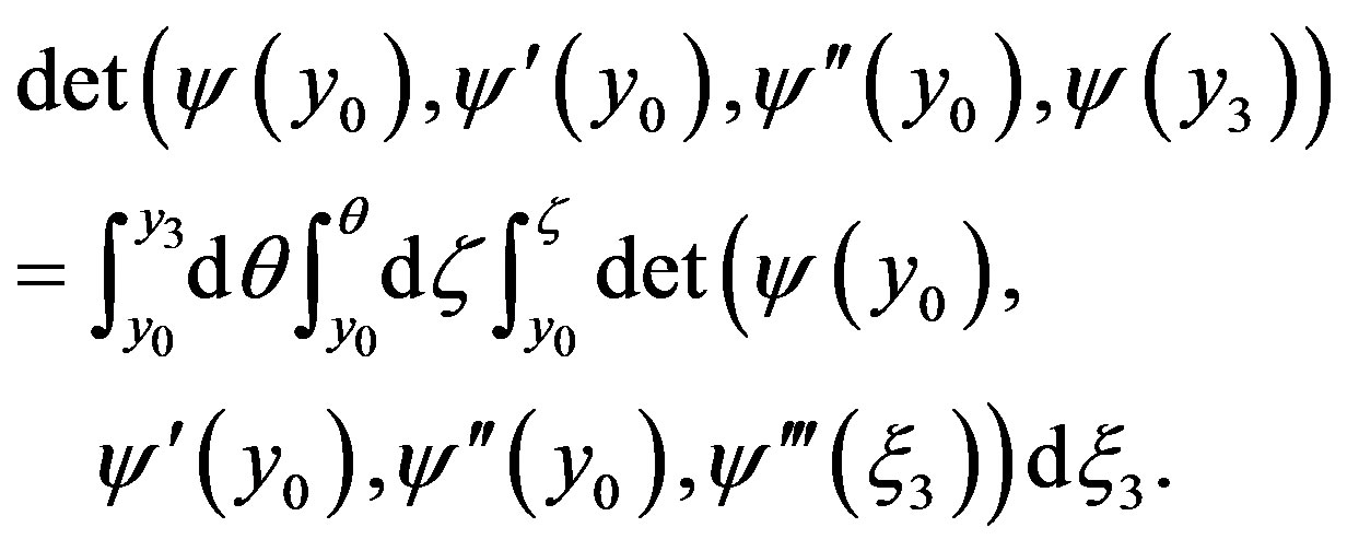
Using the additivity property of determinants and integrals and applying the Newton?-Leibnitz formula, we find
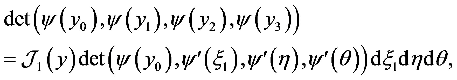
where ,
,
 (15)
(15)
Similarly,
where
 (16)
(16)
Finally
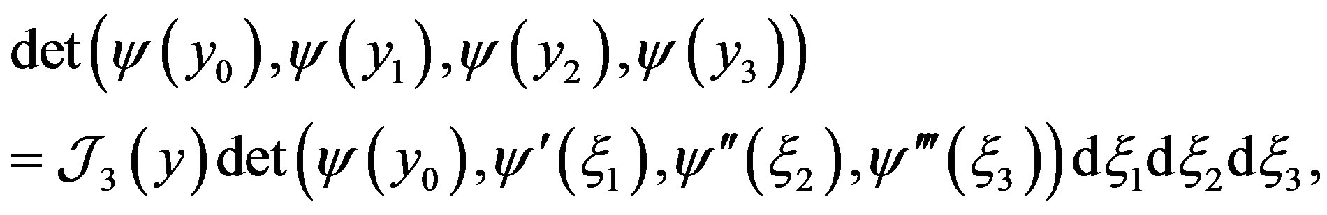
where
 (17)
(17)
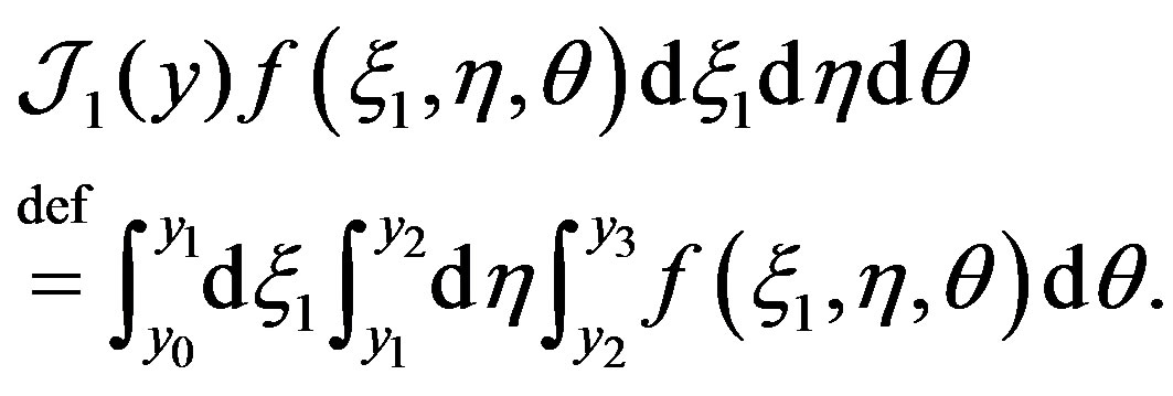
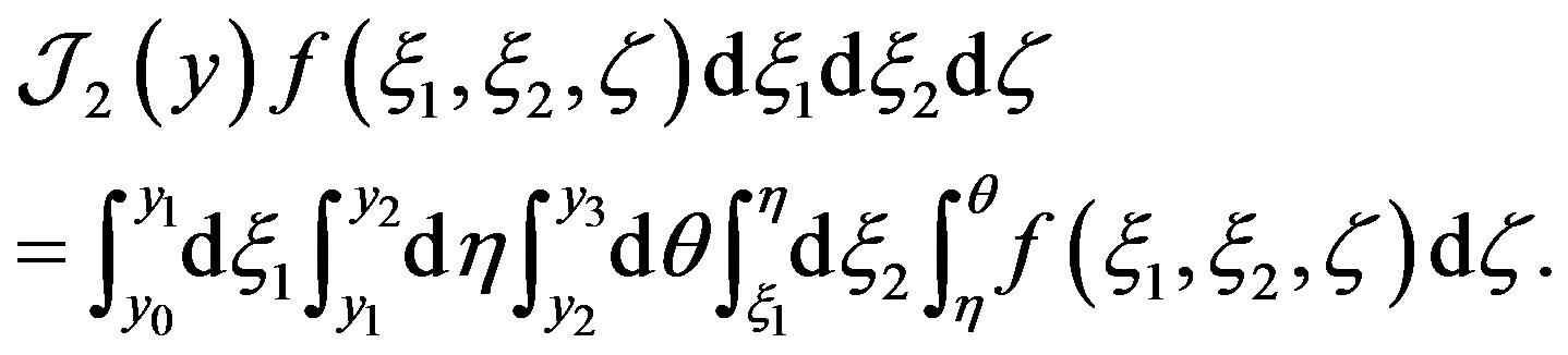
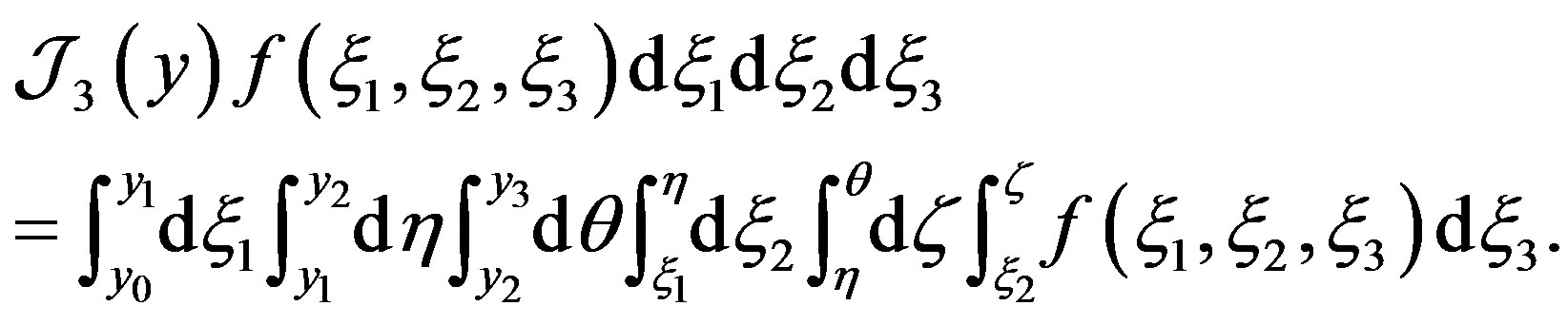
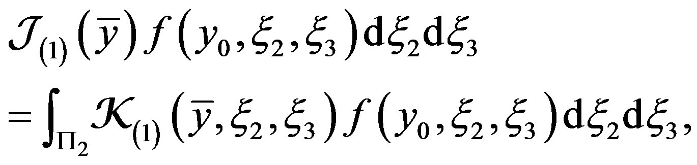
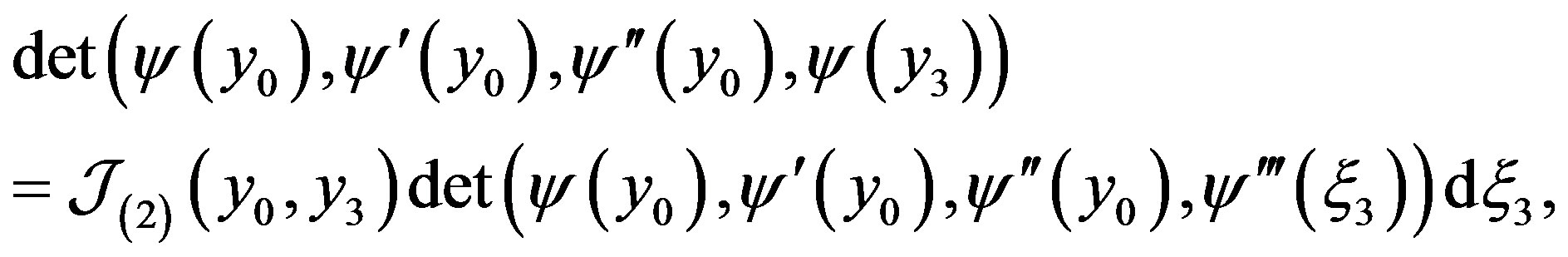
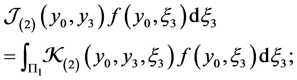
Integral operators  can be rewritten in the form
where , and
, and
 .
.
It is obvious that
 (18)
(18)
Since the lower limit is no more than the upper one in the integrals in (15)-(17), the result of integration is nonnegative for any nonnegative continuous function . Hence the integral operations
 , have nonnegative kernels By (17) we have
 (19)
(19)
Recall that vector-function  is continuously differentiable in neighborhood of the point
 , and passaging to limit as
 , we get
 (20)
(20)
It follows easily that relation (20) can be written in the form
where , and the operator
  is defined by identity
 (21)
(21)
By relations (18) and (21) we see that the integral operator  may be represented in the form
where , and
, and  is nonnegative function Taking into account (14), we obtain
  , where
 ,
,  ,
, . Thus the assertion is true in discussed case.
Now consider the case of ,
,  ,
, .
.
Let  is new variable,
 ; by definition put
 (22)
(22)
so that .
.
Under condition  according to Taylor formula we have
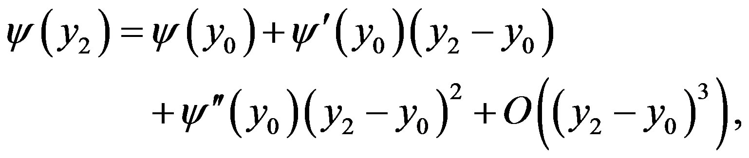
whence we get
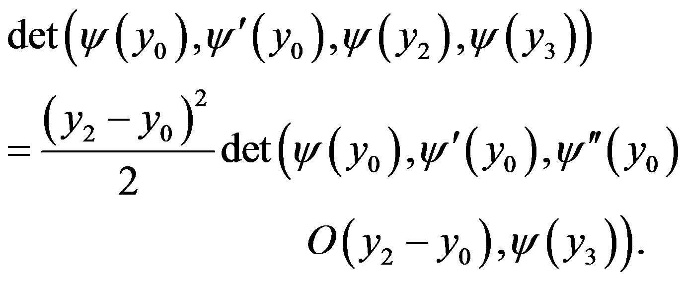
Thus by (21) we obtain
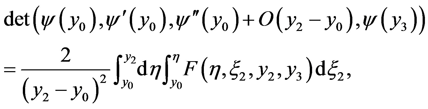
where
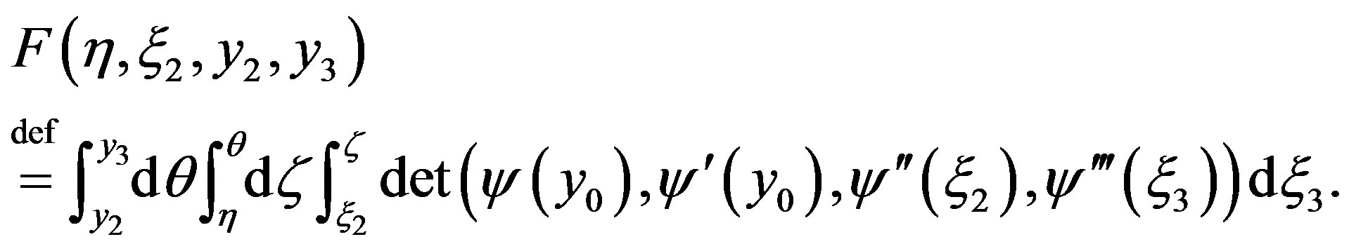 (23)
(23)
It follows in the standard way that
where ,
, .
.
Passaging to limit under  we obtain

taking into account (23), we rewrite the formula in the form
Thus
where
here 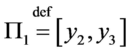 and
and  is nonnegative function.
Now recall notation (22); we obtain  , where
 ,
, . This completes the proof in discussed case.
For an arbitrary natural  one can obtain a similar representation via multiple integrals with the lower integration limit less than the upper one. Analogously the assertion is proved for
 . This completes the proof.
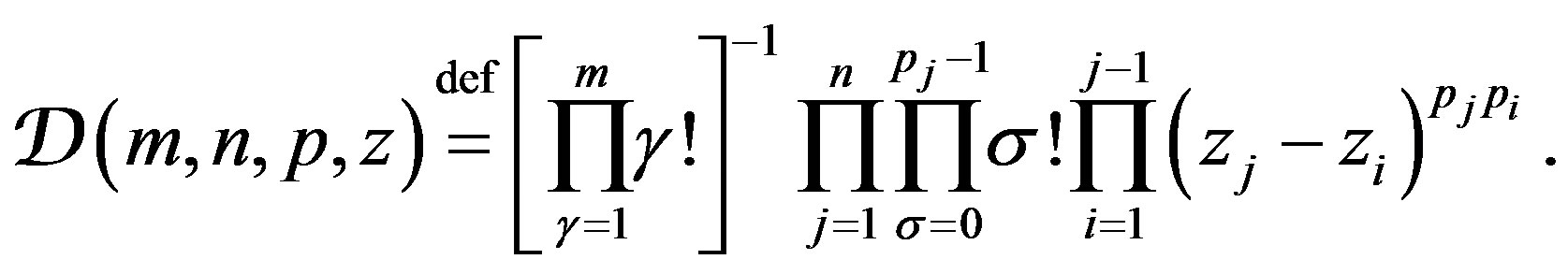
Denote  and introduce the function
Lemma 2 If suppositions of Lemma 1 are fulfilled, then
 (24)
(24)
Proof Substituting vector-function  for
for  in (13), we have
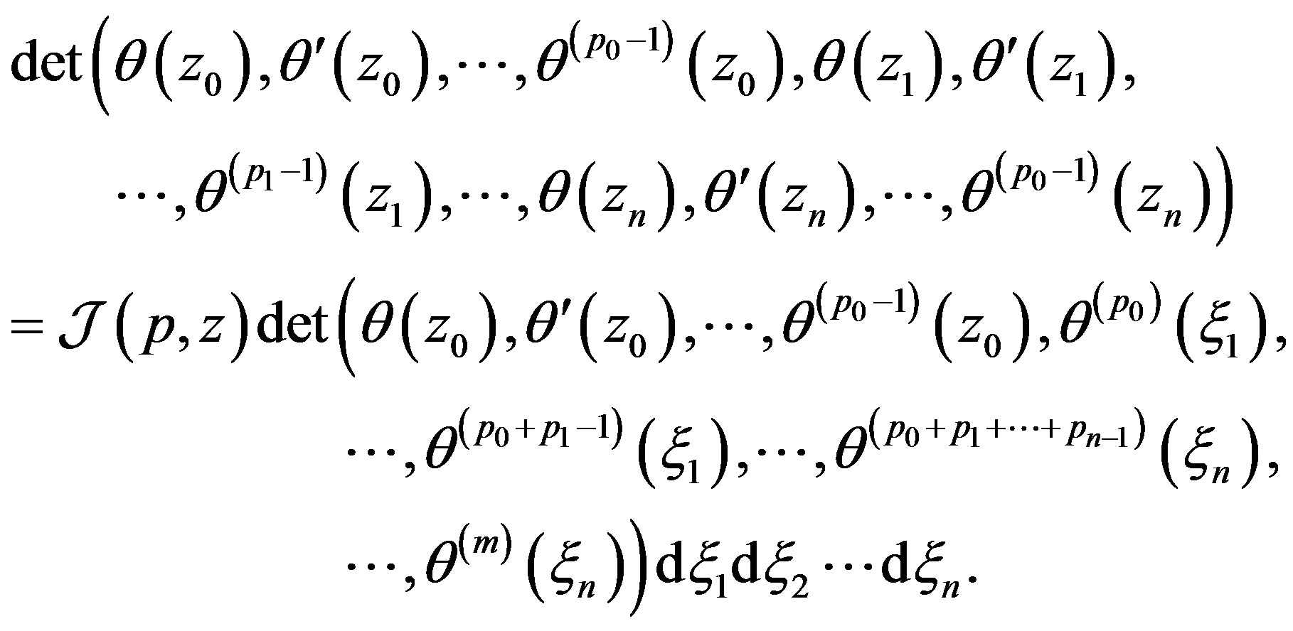 (25)
(25)
The determinant on the right-hand side of (25) contains a lower triangular matrix with entries  at the main diagonal so that right-hand side is equal to
 (26)
(26)
The left-hand side contains the determinant of matrix, which appears in Hermite interpolation problem
where  are prescribed numbers and
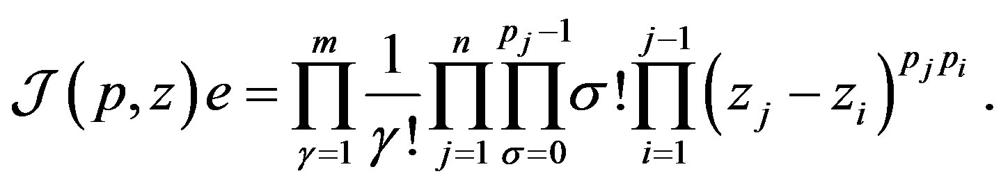
 . Value of the mentioned determinant is known (see [3], p. 43); it is equal to
 (27)
(27)
Equating of (26) to (27) gives (24). It completes the proof.
4. Evaluations of Approximation by Splines of Hermite Type
We assume that  and
and
 (28)
(28)
By the uniform continuity of the function under consideration on [a,b], from (28) we conclude that for any  there exists
  such that for
  and
and 
 (29)
(29)
where .
.
By definition, put
Lemma 3 Under the assumption (29), for  the inequality
 (30)
(30)
is true; here ,
,  ,
,  ,
, .
.
Proof We use Lemma 1 and represent  in the form (13) for
 ,
,  ,
,  ,
,  ,
, . As a result, we find
Using the estimate (29), the positiveness of the kernel of the integral operation , and the relation (24) obtained in Lemma 2, we derive the estimate (4.3) for
 .
.
Now we set
 (31)
(31)
 (32)
(32)
 (33)
(33)
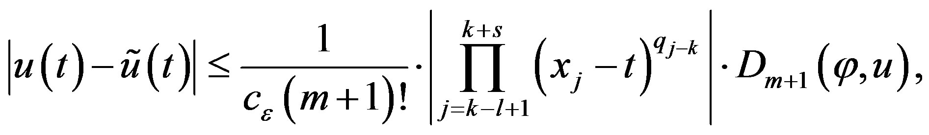
Lemma 4 If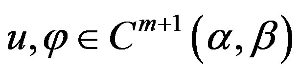 , then for
  the following inequality holds:
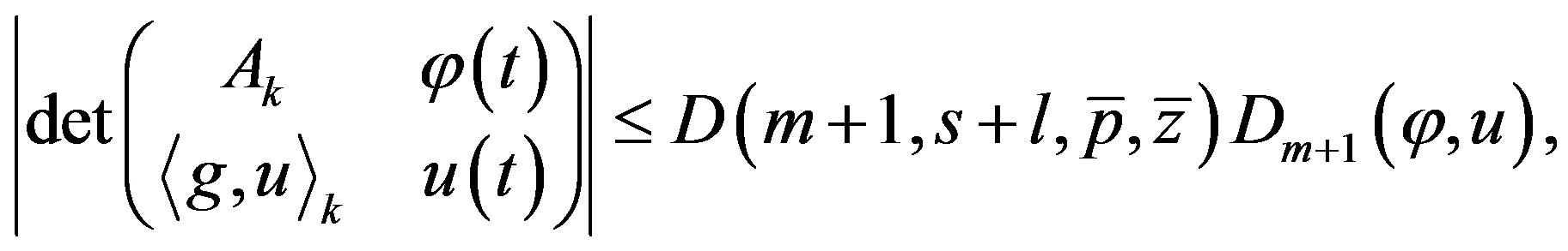 (34)
(34)
where
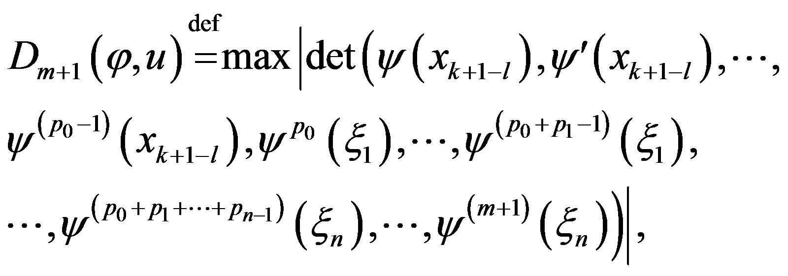 (35)
(35)
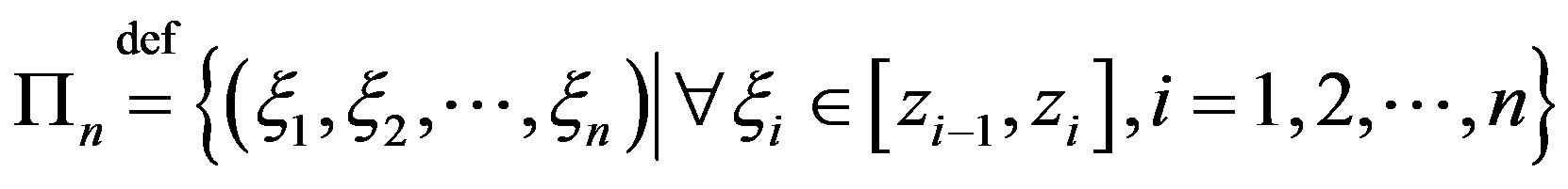
and the maximum is taken over
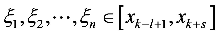
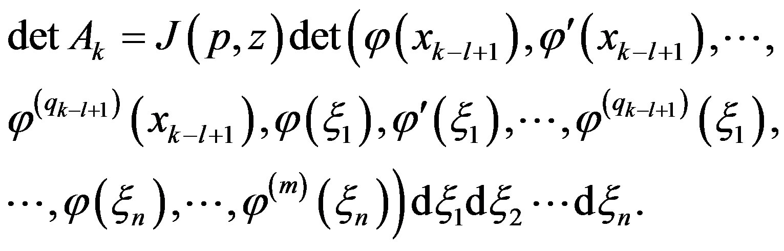
Proof By (31)-(33) the relation (13) may be written in the form
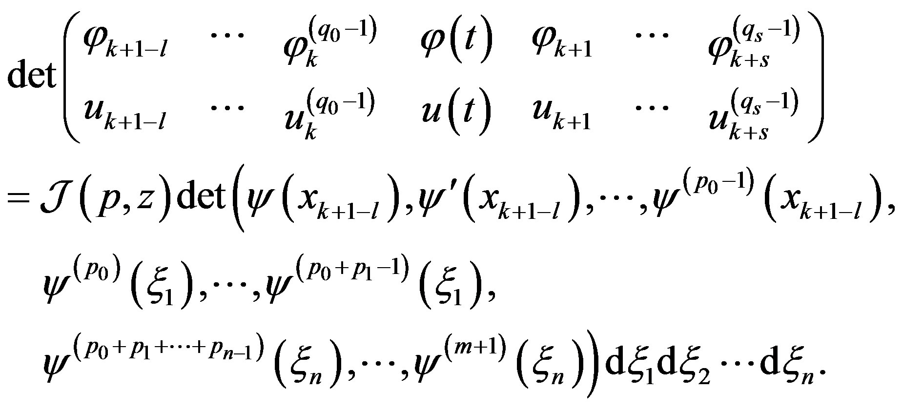
It is clear that conditions of Lemma 1 and Lemma 2 are fulfilled, and therefore the kernel of integral operator  is nonnegative. By Lemma 2 we get evaluation (34)-(35).
Theorem 3 If  and (29) holds, then for
 (36)
(36)
where  is defined by (35)
Proof Usage (34)-(35) in (12) gives the evaluation (36).
Corollary 1 Under the assumptions of Theorem 3, the interpolation  of a function
  is exact on elements of the space
 , i.e.,
 (37)
(37)
Proof If identity  is fulfilled for a number
 ,
,  , then in (33) the determinant
  includes two identical rows; therefore
 . Thus the relation (37) is true.
5. Acknowledgements
The work is partially supported by the Russian Foundation for Basic Research (grant No. 13-01-00096).
REFERENCES
- Yu. K. Dem’yanovich, “Approximation by Minimal Splines,” Journal of Mathematical Sciences, Vol. 193, No. 2, 2013, pp. 261-266.
- I. G. Burova and Yu. K. Dem’yanovich, “Theory of Minimal Splines,” St.-Petersburg University Press, St.-Petersburg, 2000.
- A. O. Gelfond, “Calculation of Finite Differences,” Nauka Press, Moscow, 1967.