Applied Mathematics
Vol.3 No.9(2012), Article ID:22993,15 pages DOI:10.4236/am.2012.39143
Characterizing Placental Surface Shape with a High-Dimensional Shape Descriptor
1Department of Mathematics and Statistics, California State University, Long Beach, USA
2Placental Analytics LLC, New York, USA
Email: jen-mei.chang@csulb.edu, amycora@gmail.com, carolyn.salafia@gmail.com
Received July 18, 2012; revised August 18, 2012; accepted August 25, 2012
Keywords: Signed Deviation Vector; Placenta; Shape Analysis; Linear Discriminant Analysis; Principal Component Analysis
ABSTRACT
The human placenta nourishes the growing fetus during pregnancy. The newly developing field of placenta analysis seeks to understand relationships between the health of a placenta and the health of the baby. Previous studies have shown that the median placental chorionic shape at term is round, and deviation from such prototypical shape is related to a decreased placental functional efficiency. In this study, we propose the use of a nearly-continuous shape descriptor termed signed deviation vector to systematically study the relationship between various maternal and fetal characteristics and the shape of the placental surface. The proposed shape descriptor measures the amount of deviation along with the direction of the deviation a placental shape has away from the shape of normality. Using Linear Discriminant Analysis, we can independently examine how much of the placental shape is affected by maternal, newborn, and placental characteristics. The results allow us to understand how significantly various maternal and fetal conditions affect the overall shape of the placenta growth. Though the current study is largely exploratory, the initial findings indicate significant relationships between shape of the placental surface and newborn’s birth weight as well as their gestational age.
1. Introduction
The human placenta is a fetus’s lifeline during gestation, providing nutrients and antibodies, while eliminating waste products via the mother’s blood supply. The placenta is an integral part of the child’s development, but is generally disposed of after delivery. The relatively new field of placenta analysis within the field of perinatal pathology investigates the possibility of learning important health information about the child from the placenta. The theory is that the placenta may hold vital information that can contribute to clinical practice and patient care.
The placenta is connected to the uterine wall and exchanges nutrients and waste through the placental blood barrier. It connects to the fetus by the umbilical cord containing two arteries and one vein. The cord inserts into the chorionic plate, or fetal side of the placenta, where the vessels branch into a network covered by a thin layer of cells. This vascular network is one area that placenta analysts continue to research. Similar to the root system of a tree, the vascular network must effectively and efficiently provide nutrients for the fetus as it grows larger. Intuitively, the optimal network would have the base of the umbilical connection in the center where vessels branch evenly and thoroughly in all directions. Previous studies by [1] have found that the average placenta is in fact structured optimally with round placentas having the umbilical cord centrally inserted.
Additional studies have found that the directional growth of the vascular network influences the final shape of the placenta. For example, if the uterine environment limits the growth of vessels, the placental shape will reflect the obstacle, as illustrated in [2]. Currently, the causes of placental shape irregularity are not fully understood. Furthermore, medical understanding of the effects of irregularly shaped placentas and poor vascular coverage is also limited.
In this study, we search for connections between the geometric shape of the placenta and physical features of the mother, fetus and placenta. During the investigation, we confirm prior results finding the average placental shape to be round with the umbilical cord centrally located. Also, we develop a measure to numerically represent a placenta’s geometric deviation from the average shape. The proposed shape descriptor can then be employed to analyze any maternal, newborn or placental feature.
We begin in Section 2 with a description of the data sets used in this study. In Section 3, we describe the steps taken to preprocess and register the given placenta images in order to perform computations without introducing bias. We propose a numerical shape descriptor to measure the amount and direction of deviation of a given placental surface shape away from a normal placental shape in Section 4. Linear Discriminant Analysis is used in this study to reveal a suggestive relationship between the shape of placental surface and various medical features. For completeness, a brief overview of the discriminant analysis will be given in Section 5. The discriminating power of the proposed shape descriptor is revealed under a series of carefully designed experiments and the mathematical and medical implications of those experiments will be described in Section 6. Finally, concluding remarks and future areas of research are given in Section 7.
2. Materials
2.1. Digital Images
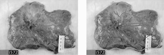
There are two data sets investigated in this study. The first data set is a subset of a collection of 1225 digital photographs of placental surfaces and their accompanying medical data. This information originated from the Pregnancy, Infection, and Nutrition Study at an academic health center at the University of North Carolina (UNC). The data set is fully described in [3] and made available by Placental Analytics LLC. Each of the 1225 placentas went through a consistent protocol of cleaning and trimming of extra placental membranes and umbilical cord before being photographed with a standard high-resolution digital camera. The minimum image size is 2.3 megapixels. The placentas were oriented prior to being photographed so that the point on the perimeter closest to the rupture point on the amniotic sac was placed on the negative vertical axis for consistency. This orientation is the best approximation to the orientation the placenta took in the uterine environment prior to delivery, and thus is biologically significant as indicated in [1]. Each placenta was photographed with either a ruler or a penny for scaling purposes within the field of view. Examples of the original images can be seen in Figure 1.
Of the 1225 placentas photographed, 150 were traced by hand by a trained pathologist. Fifty images were chosen at random from each group of low, normal and high birth weights according to the following criteria. Birth weights below 2500 grams are considered low, weights above 3500 grams are considered high, and those in between are considered normal. Different criteria for labeling birth weights are described in Section 2.2. Using a Tablet PC and GNU Image Manipulation Program (GIMP)the perimeter was traced in green, the umbilical cord insertion marked in yellow and the blood vessels traced in pink. While automatic vessel extraction and perimeter detectors are being developed by, e.g., [4], they are still far from perfect for this data set. Therefore, we select the 150 hand-traced images to be the ground truth for the perimeter shape and the vascular structure. Four of the tracings were poor, one was a duplicate, four were missing placenta weights and two were missing a maternal vascular pathology diagnosis. Thus, the first data set investigated in this study includes  cases, which are 93% of the traced set and 11% of the original set. Figures 2(a) and (b) show the original and traced images, respectively, of one placenta from this set.
The second set of data, termed the NYU data set, comes from a collection of 96 placenta images from New York University. The placentas were trimmed, cleaned, and oriented prior to being photographed, consistent with the treatment of the placentas from the Pregnancy, Infection, and Nutrition Study in North Carolina. All 96 of these images were hand-traced by the same trained pathologist, following the same procedure and protocol as described before. Of the 96 cases, twelve were missing the placenta weight and three were missing gender labels. Thus this data set includes  cases, which are 84% of the original collection. Figure 3 shows an example of one placenta from this set.

Figure 1. Example images from the original UNC data set.
 (a) (b)
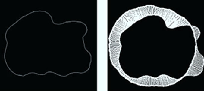
Figure 2. (a) Image of placenta ID#1572 from the UNC data set; (b) Traced image of placenta ID#1572 from the UNC data set.
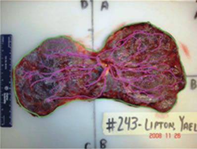
Figure 3. Image of placenta ID#243 from the NYU data set.
2.2. Medical Features
The maternal data used in this study includes: 1) mother’s age at the beginning of pregnancy and whether or not the mother suffered from 2) eclampsia or preeclampsia, 3) gestational diabetes, 4) chronic hypertension, or 5) pregnancy-induced hypertension. The newborn data includes the 6) birth weight in grams, 7) gender, and 8) gestational age measured in weeks. Under the supervision of Dr. Carolyn Salafia, technicians at Early Path Clinical and Research Diagnostics, a New York Statelicensed histopathology facility, performed image analysis, a histology review and a gross examination of each placenta. The pathology exam resulted in six diagnoses of the pathology of each placenta, which were recorded as either present or not present. Thus the placenta data includes the presence or absence of 9) acute inflammation, 10) chronic inflammation, 11) vascular pathology, 12) maternal vascular pathology, 13) fetal vascular pathology, and 14) other vascular pathology. Detailed histopathological diagnoses are described in [5].
Each of the two data sets of images is accompanied by the birth weight in grams, gender, and gestational age in weeks. In the case of the UNC data set, there are eleven additional features listed previously.
In this preliminary study, we require that each of the features has a two-class label. That is, for any given medical feature, it can be categorized as one of two options. The presence of eclampsia or preeclampsia, gestational diabetes, chronic hypertension and pregnancyinduced hypertension in the mother already have this dichotomy. A present condition is labeled as 1, and not present is 0 except that gender is divided so that male is labeled as 1 and female is given a 0. Similarly, the six vascular pathologies are labeled 1 for present and 0 for not present. When the mother’s age at the beginning of pregnancy is 35 or more, the mother is labeled as having advanced maternal age (AMA). Such cases are labeled 1, while mothers beginning pregnancy under the age of 35 are labeled 0. Pregnancies that lasted less than 37 weeks of gestation are labeled as preterm with a 1, while pregnancies that reached or exceeded 37 weeks are labeled term with a 0.
Furthermore, the birth weight is also labeled, but medical resources mainly classify in a three-class system of low, normal, and high birth weights. Realistically speaking, the low birth weights are considered to have the highest health risk while babies who are born with normal or high birth weights are less likely to develop threatening health conditions. Because of this, cases of normal and high birth weights are grouped together and given the label “Not at Risk” and numerically represented by 0, while cases of low birth weight are labeled “At Risk” and numerically represented by 1. Initially the birth weight (BW) data came separated according to the piecewise labeling rule  such that
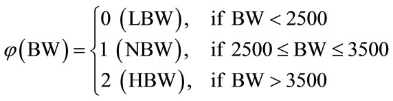
It is henceforth referred to as Labeling Scheme I. This labeling, however, does not take into account the gestational age of the newborn. Naturally, a shorter gestation will lead to a lower birth weight, so the region of normalcy must be adjusted based upon the gestational age in weeks. Two additional labeling options are presented next. An important aspect of this study is to search for a superior labeling scheme to be implemented in medical practice that has the most practical uses.
Williams Obstetrics [6], a central text in the medical specialty of obstetrics, provides a table of percentiles for birth weights and gestational age. The table is based on 3,134,879 single live births in the United States. It includes the fifth, tenth, fiftieth, ninetieth and ninety-fifth percentiles for birth weights of children born between the twentieth and forty-fourth week of gestation.
The table is used to create two other labeling options: Labeling Scheme II uses the 10 - 90th percentile range as normal, and Labeling Scheme III uses the 5 - 95th percentile range as normal. The advantage of using these labeling schemes is that the percentiles in the table come from a large data set of over three million live births. The disadvantage, however, is that these labeling schemes label all children born before the 35th week of gestation in our study as normal.
There are a combined total of 1099 unique placentas from the two original data sets together with corresponding birth weights and gestational ages. Table 1 shows the number of placentas classified in the categories of low birth weight (LBW), normal birth weight (NBW), and high birth weight (HBW) for each labeling scheme. The proposed shape descriptor will then be used to investigate the level of discriminatory power inherited within these three labeling schemes.
3. Data Registration
In this section, we will describe the steps required for
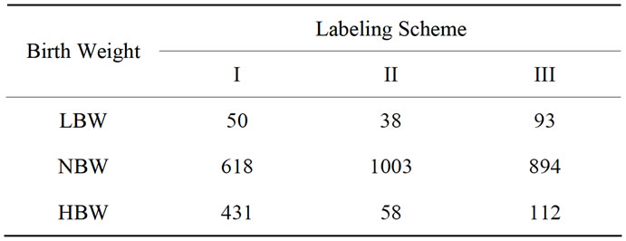
Table 1. Number of placentas that are categorized into each birth weight group in the original UNC data set for the three labeling schemes.
preprocessing the images from the UNC and NYU data sets. The traced images from the UNC and NYU data sets were conveniently oriented, however, it was still necessary to preprocess the images to properly scale them and extract the perimeter shapes. This work was done using MATLAB and ImageJ, an image-processing program provided by the National Institutes of Health. While missing medical features limited our sets to  and
and , 143 images from the originnal UNC set and all 96 from the original NYU set remain useful images. Maximizing our image database was beneficial for future computations of median placenta shape to be discussed in Section 4.1. Therefore, the preprocessing steps described in this section are applied to a total of 239 traced images.
Black and white digital photographs of length n by height m are represented in MATLAB as m-by-n matrices with integer entries between 0 and 255. The entries take these values because each pixel of the image is stored in 8-bit, so there are  possible intensity values. Zero intensity corresponds to black and an intensity of 255 corresponds to white. Since the images are in color, three sets of intensities are stored in the red, green, and blue channels. The 143 images of placentas from the UNC set ranged in size from 1024-by-768 to 1600-by- 1200. All images were first normalized to size 1600-by- 1200 for the ease of future computations. Similarly, the 96 images from the NYU data set ranged from 2228-by- 1587 to 3008-by-2000. Similarly, smaller images were padded to be 3008-by-2000 to obtain a database of images with consistent resolution. Figure 4(a) shows placenta 1618 from the UNC data set padded to be 1600- by-1200.
Since the images were not taken from the same height with the same zoom, it was necessary to scale the images before performing other computations. Each image included either a piece of a ruler or a penny. Using ImageJ, we recorded the number of pixels present in one centimeter on the ruler or along the diameter of the penny, thus providing a scale for each placenta.
Next, using MATLAB, the boundary of the placenta was extracted from the green perimeter hand tracing and filled with white to form the placental mask. The resulting matrices are 1600-by-1200 or 3008-by-2000, for the appropriate data set, consisting of ones where the placental surface exists and zeros outside of the placenta boundary. Also, we extracted the umbilical cord insertion point from the yellow tracing. The mean of the yellow pixel locations provided a single point for the umbilical insertion. Figure 4(b) shows the result of this step.
Now with the scale, umbilical point and the masks, the images could be scaled to two pixels per millimeter and translated such that the umbilical insertion point rested in the center of each image. Notice that the umbilical cord insertion point was chosen as the center of the image, as opposed to the geometric center of the placenta shape, since the geometric center has no particular significance in the internal structure of the placenta as indicated in [7], and has been shown to have no significant correlation with the functional efficiency of the placenta.
With each of the images scaled and centered about the umbilical cord insertion point, the images are ready for analysis. After the scaling, however, the placental masks and boundaries do not need matrices of size 1600-by- 1200 or 3008-by-2000 to contain the important chorionic plate information. A minimal bounding box of size 797- by-1049, computed from all placental masks, was then
 (a)
(a)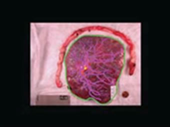 (b)
(b) (c)
(c)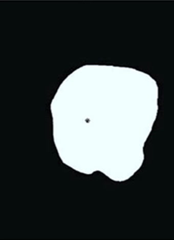 (d)
(d)
Figure 4. An illustration of preprocessing on placenta ID#1618. (a) Traced image is first padded with zeros to reach the desired resolution; (b) Placenta mask and umbilical cord location are extracted; (c) Image from (b) is scaled and aligned so the umbilical cord insertion point appears in the center of the resulting image; (d) A one-pixel boundary of the placental surface.
imposed on each image to reduce computational complexity. As shown in Figure 4(c), all matrices are thus reduced to 797-by-1049 with umbilical cord insertion points still at the center, (399, 525), of the images.
In some instances, the entire mask of the placental surface, also referred to as the chorionic plate, is required for analysis. At other times, the boundary, one pixel in width, is sufficient. For future analysis, the images are eroded to the boundary matrices, still of size 797-by- 1049 as shown in Figure 4(d).
4. Placental Surface Geometry
This study seeks to investigate which of the features collected for the given data sets are most connected to the geometric shape of the placenta.
Previous studies have shown that an average placenta is round with the umbilical cord inserted in the center. Also, deviation from the prototypical placenta shape is related to a decrease in placental functional efficiency as illustrated in [1]. To study the potential relationships, it is important to have a reliable and accurate mathematical representation for the shape of the placental surface. Together with a shape representing normality, the accurate representation of the shape can provide a numerical measure of deviation from normality. In this section, we propose a nearly continuous shape descriptor that can be made to measure the deviation from normality to any degree of precision as desired to study the relationship of shape and various medical features. While our feature list is limited, our hope is that the calculation of the proposed shape descriptor can be automated and the results can be used in future placenta studies with more extensive medical data about the child’s health.
We begin the section by forming the median placenta shape for the combined set of traced images from the UNC and NYU data sets. We then describe the proposed shape descriptor called the signed deviation vector for the placentas in the UNC and NYU data sets.
4.1. Shape of Normality
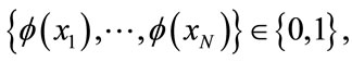
The resulting 797-by-1049 image matrices obtained from the registration process in Section 3 include the surface masks of the 239 hand-traced images and their respective eroded boundaries. Following a similar procedure referenced in [5], this section describes the definition and creation of the median placenta shape using those 239 masks.
Mask matrices,  , where
 , contain zeros where there is no appearance of placental surface, while ones mark the coverage of the chorionic plate. For any given pixel or element in a matrix,
  , here
  and
and  the number of times a placenta occurs at that location, over all images, is recorded in the frequency matrix,
 . Notice that in our experiments,
  and
and . Thus,
The values at each position of  can range from 0, meaning no placenta ever appears at that pixel, to N, where all the placentas agree. For example, since all the images have the umbilical insertion point translated to the center of the image matrix (399, 535), it must be true that in our data set
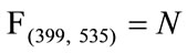 . The resulting frequency matrix is shown in the leftmost plot in Figure 5 where the brightest white corresponds to
 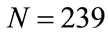 and black corresponds to zero. The median shape mask is defined by the m-by-n matrix
  where
where
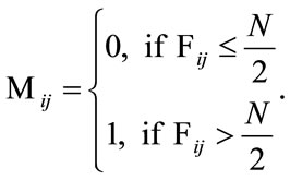
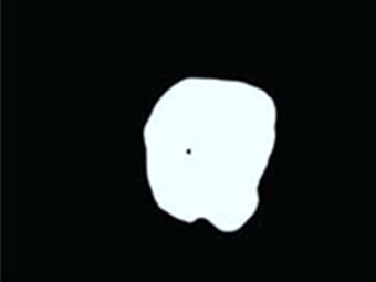
This means that if over half of the contributing placentas occur at a given pixel, then that pixel is considered part of the median shape. The boundary where the frequency reaches N/2 is shown in the middle plot of Figure 5 and the final median placental shape,  , is shown in the rightmost plot of Figure 5.
The area of the median placenta is Amediam = 100,588 pixels which amounts to 251.5 cm2. The centroid, or the geometric center of mass, lies at (403, 535), and is marked in the rightmost plot of Figure 5 with an asterisk. It lies very close to the actual center of the image (marked with a circle), which is the shared umbilical cord insertion point for the contributing placenta shapes. The area, if associated with a perfect circle, would result in the radius being 8.95 cm. If we overlay a best-fit ellipse on top of , then the major axis length is 18.7 cm, the minor axis length is 17.1 cm and the eccentricity is 0.39, where the eccentricity is defined to be
 , where c is the distance between foci of the best fit ellipse and a is the length the major axis. A perfect circle has an
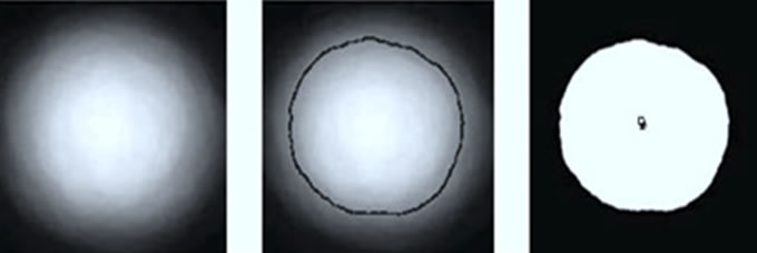
Figure 5. An illustration of the process of creating the median placenta shape on UNC and NYU data sets. Left: Frequency matrix. Middle: Separation of frequency where pixels lie within the one-pixel curve represent the majority. Right: The resulting median placenta shape. The circle gives the center of the image while the asterisk gives the geometric center of mass of the resulting median shape.
eccentricity of 0, while a straight line has an eccentricity of 1. These measurements mean that the median placenta shape is approximately circularwith the umbilical insertion point at the center and a radius of approximately 9 centimeters. This result is in accordance with previously documented results shown in [5].
The median shape in the rightmost plot of Figure 5 is a combined product of the 239 masks from the UNC and NYU data sets. It represents the shape of normality for these two sets, and will contribute to the formation of the shape descriptor for each placenta. The next section describes the formation of the proposed signed deviation vector that will measure the deviation from the median shape.
4.2. Shape Descriptor
With the median shape available for the data sets, the shape information for each placenta can be measured as its deviation from the prototypical placenta shape. We propose to capture this unique information with a shape descriptor called the Signed Deviation Vector (SDV). In short, the elements of the SDV measure the difference between the distance to the edge from the umbilical cord insertion point on the placenta and the corresponding distance measured on the median placenta shape. In general, each SDV is a k-dimensional vector. In our study, we use k = 360-dimensional signed deviation vectors for the UNC and NYU data sets calculated from the cropped 797-by-1049 boundary matrices. The derivation of the SDVs from the median shape and the boundary matrices is described next.
The one-pixel width boundary of the placenta perimeter is stored in a m-by-n (m = 797, n = 1049 in our case) matrix of ones where boundary exists and zeros elsewhere. From the matrix center,  measures the angle counterclockwise from the positive x-axis and is measured in one degree increments from 1 to 360. Radial coordinates,
  , are defined to be the coordinates of the boundary at
 . A radial distance,
  , is defined to be the distance, in pixels, from the center of the image,
  (x0 = 399, y0 = 525 in our case), to the radial coordinates,
  so that
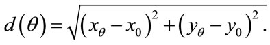
Figure 6 gives a visual representation of the radial distance. For a placenta,  the radial distances form a 360-element vector
  with elements of the nth image. Similarly, since the median boundary is obtained by taking the one-pixel boundary of the median placenta, the vector
  holds the radial distances for the median shape.
Now, the signed deviation vector,  , for a given placenta,
  is defined by
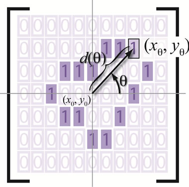
Figure 6. An illustration of the radial distance.
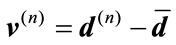 . (1)
. (1)
This forms a 360-element vector with positive elements corresponding to radial coordinates on the placenta that are farther from the center than the median shape’s radial coordinates.
The SDV is a unique way to measure the nearly continuous deformation of a shape from a fixed contour, henceforth a powerful tool in describing the discriminatory feature of a shape contour. On the other hand, measures that rely on a single number such as the symmetric difference of areas [7], do not guarantee uniqueness of shape which makes it harder to draw conclusions from the results. We show in Lemma 1 that the uniqueness of SDV can be extended to any convex closed curve.
Lemma 1. Let the radial distance,  , be the Euclidean distance from the radial coordinate
  emanating from the center of the coordinate system
  so that

Furthermore, suppose  takes on values from a family of ordered real numbers between 0 and
 ,
, . A radial distance vector, d, can be formed for a given convex closed curve such that
 . Then the signed deviation vector for this curve, defined by
 , is unique, where
  is the radial distance vector for a fixed contour.
Proof .Suppose the contrary that two distinct convex closed contours,  and
and , have the same SDV, then
where  and
and  are the radial distance vector for
  and
and , respectively. This implies that
  and
and  must agree for all
  That is, for any
 ,
,
 (2)
(2)
Since  and
and  are convex and v is signed, there exist unique
  such that
and
If  the uniqueness is trivial. Therefore, we assume
  Thus, along with Equation (2), we have
whichreduces to  or
or .
.  can not be
  due to positivity. Hence,
  which results in
  and consequently
  agrees with
  completely on
  This is a contraction.
Figures 7(a) and 8(a) illustrate the boundaries of placentas 243 and 1572, respectively. Their SDVs can be visualized in Figures 7(b) and 8(b) as the distances represented by the arrows starting at the radial coordinates on the median shape,  , and ending at the corresponding radial coordinates on the placenta. The median shape is slightly thicker. Arrows pointing outward represent positive elements in the SDV, while inward-pointing arrows represent negative elements.
Geometrically, these two SDVs capture distinct variations. For example, majority of the elements in  have negative value while roughly half of the elements in
  are negative indicating that
  is smaller than
  while
while  is likely to be elongated. Moreover,
 (a)
(a)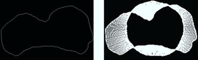 (b)
(b)
Figure 7. A Visualization of the signed deviation vector for placenta ID#243. (a) Boundary of P(243); (b) SDV of P(243).
 (a) (b)
Figure 8. A Visualization of the signed deviation vector for placenta ID#1572. (a) Boundary of P(1572); (b) SDV of P(1572).
i.e., the the overall magnitude of  is much larger than the overall magnitude of
 . Combining these two pieces of information, we can conclude that
  is much larger than
  and
and  is quantitatively less round. Evidently, the newborn who is associated with
  weights 1600 grams while the newborn who is associated with
  weights 3360 grams. Under all three birth weight labeling schemes,
  is labeled as a “At Risk” and
  is labeled as a “Not at Risk”. Using the proposed signed deviation vectors, we can capture how the shape and size of a given placenta varies from the geometry of what considered as a normal placenta under a specified medical label.
5. Methods
To empirically test the validity of the proposed shape descriptor (signed deviation vector) in gauging variation exhibited in the maternal and fetal features, we performed a series of analysis. First, Principal Component Analysis is used to reduce the high-dimensional shape information to a manageable and meaningful size. This step is a cautionary measure to avoid the issue of overfitting that is commonly associated with LDA for an under-sampled problem [8,9].
The PCA step is followed by a correlation analysis to gain a rough intuition for whether the shape descriptor is a good proxy for studying maternal and fetal conditions. Once a suggestive correlation is established, we use Linear Discriminant Analysis (LDA) to examine latent shape structures exhibited in distinct groups of medical conditions that can be explained linearly. The results from LDA comprise the heart of this study and will be presented in Section 6. Here, we explain briefly how information extracted from PCA can be used in this context and give a quick overview of LDA for our purposes.
5.1. PCA
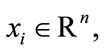
Let  be a set of distinct placentas. For each
 , associate it with an m-dimensional signed deviation vector,
  , that becomes distinct columns of the data matrix X. Note that the order at which these vectors are listed does not affect the outcome of this computation. After the data set is centered at the origin of the coordinate system, a singular value decomposition of X is performed next to obtain a set of optimal orthonormal basis,
 ’s, spanning the space where
 ’s reside. The coefficient, i.e., magnitude of the projection, of each
  onto the ith basis,
  , is given by the inner product
Intuitively, the first principal direction,  , represents a feature that the majority of the group members share. For example, for a set of colored circles, the first principal component when displayed as an image will look like a circle without color. In another word, the first few principal components of a data set offer the dominant directions of intrinsic features and the corresponding coefficients show how much of a certain feature is exhibited in the data point.
The projected coefficient,  , of the
  subject in the ith principal direction provides shape information for the
  subject in a meaningful dimension. The way these numbers capture the shape variations inherited in a given placenta is similar to how they are used in capturing face features [10]. For convenience, let
  be an n-dimensional column vector storing the coefficient of each data point projected onto the ith basis direction, i.e.
 ,
, 
Table 2 shows the Pearson correlation coefficients derived from the UNC data set between various birth weight labeling schemes and the first five projected coefficients. Notice that with 99.9% accuracy, the important shape features can be rearranged to actually lie in a 24- dimensional subspace embedded in the 360-dimensional ambient space. We draw from this information the effecttiveness of each dimension of the shape coefficient has in predicting birth weight labels.  consistently appears to have the highest correlations with all of the birth weight labeling schemes with
  and
and  showing the next layer of significance.
This result prompts us to investigate further the discriminating power of the shape coefficients ,
,  , and
, and  in predicting a maternal or fetal feature. Questions such as “is the birth weight of the newborn affected by the shape of the placenta” and “can we tell from looking at the shape of the placenta that a baby is going to have a high or low birth weight” are at the heart of the investigations.
Figure 9 provides a visualization of the UNC data points when projected down to two dimensions using the coordinates of  and
and  as well as three dimensions using the coordinates of
 ,
,  , and
, and .
.
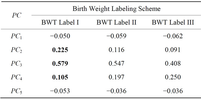
Table 2. Pearson correlation coefficients derived from the UNC data set between the first five projected coefficients and various birth weight labeling schemes.
The data points do not change their locations as we move from one row to the other; however, the labels assigned to each point vary as we switch from one labeling scheme to the next. Collectively, Figure 9 helps us assessing the optimal birth weight labeling scheme for the chosen shape descriptor. Ideally, the data points associated with each birth weight group should separate themselves from the other two point clouds perfectly in the best labeling system if shape information alone can be used to predict health risks. When this phenomenon is not observed, we need a method to measure the goodness of the linear separation. It is also worth noting that the linear separation appears to be very strong between the LBW and HBW groups, as illustrated in Figure 10. This result confirms the discriminating power of the proposed shape descriptor in the case of extreme conditions.
5.2. LDA
Linear Discriminant Analysis (LDA) is a method used in machine learning to learn a hyperplane that linearly separates high-dimensional data into disjoint sets. Considering its success in applications of face recognition [11] and the nature of the shape descriptor, we exploit it here as a first step towards understanding the interplay between the shape of placental surfaces and maternal and fetal features.
The two-class scenario of the LDA is often referred to as Fisher’s Discriminant Analysis (FDA) named after Sir R. A. Fisher, who in 1936 documented his use of a similar discriminant to classify the two flower species, Iris Setosa and Iris Versicolor [12]. Since our core task is a classification problem with binary label of “At Risk” and “Not at Risk”, FDA seems to be a natural first choice for this exploration. Briefly, given a set of points ,
,  and their corresponding class labels,
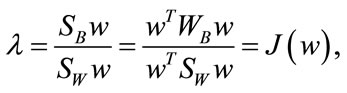
 let D0 and D1 be the set of points in D with class label 0 and 1, respectively. A line with coefficients stored in w can be learned by maximizing the Fisher criterion
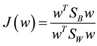 , (3)
, (3)
where SB is the between-class scatter matrix measuring the variance between the two class means and SW is the within-class scatter matrix measuring the overall variances between each point and its class mean. With classwise means defined to be
 and
and 
where n0 and n1 are the number of elements in D0 and D1 respectively, the scatter matrices can be written as
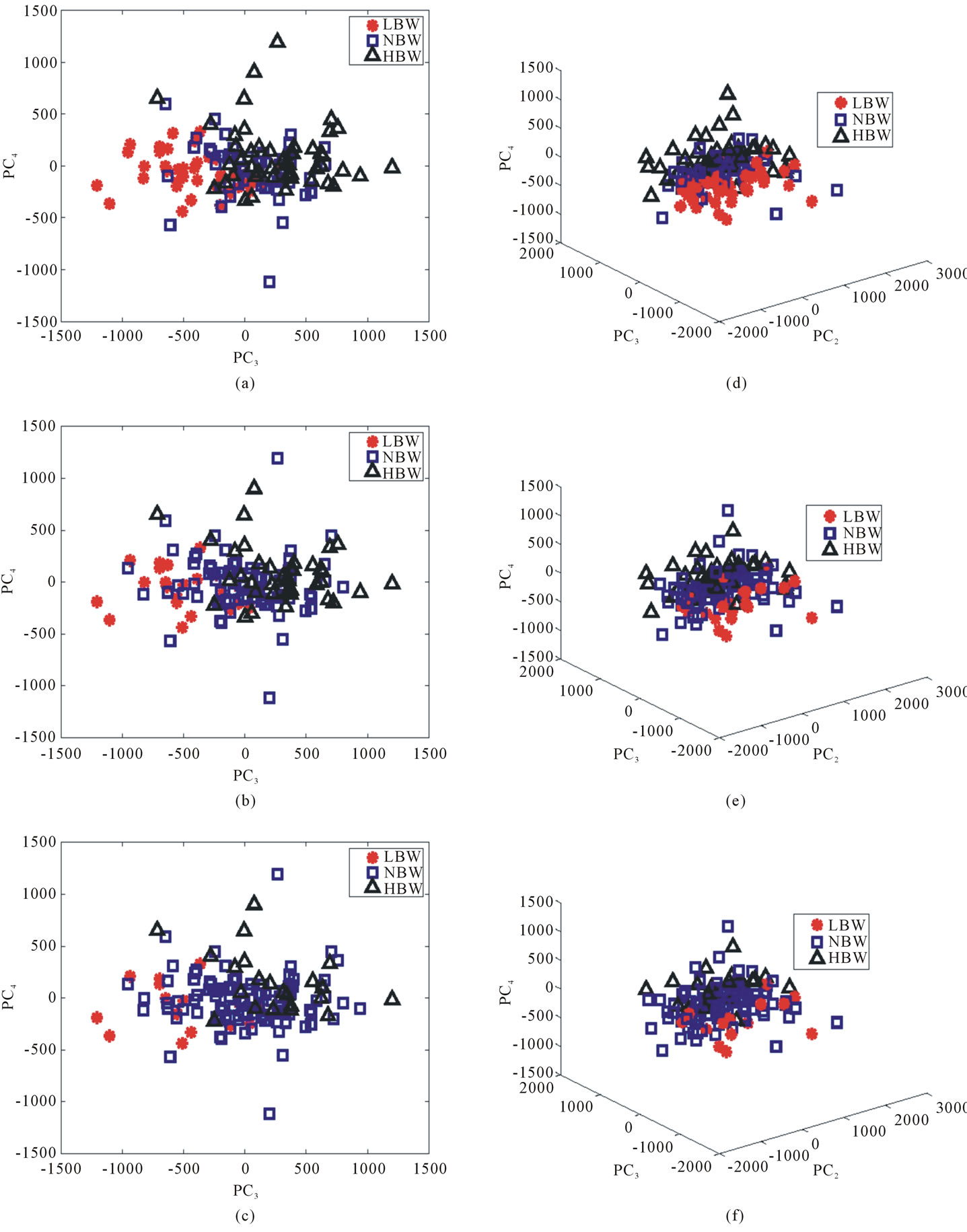
Figure 9. The signed deviation vectors for each point in the UNC data set represented in (a)-(c) PC3 and PC4 coordinates and (d)-(f) PC1, PC3, and PC4 coordinates for each of the three labeling schemes. (a) and (d): BWT Label I. (b) and (e): BWT Label II. (c) and (f): BWT Label III.
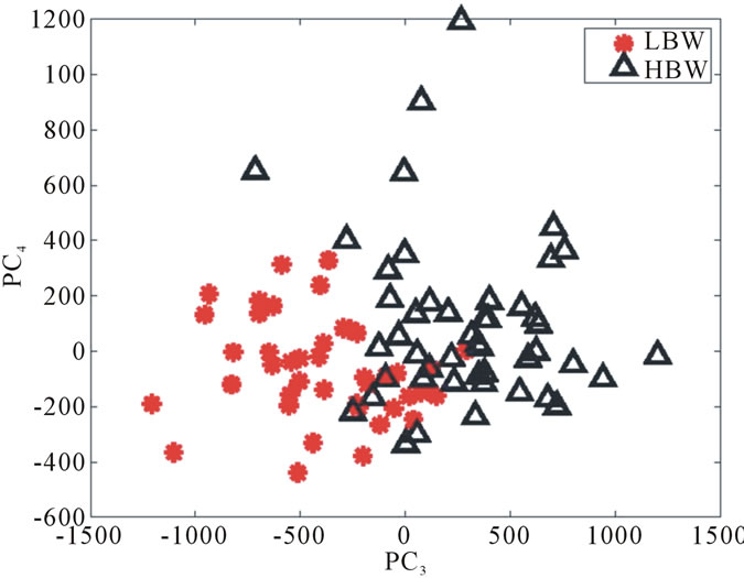
Figure 10. The signed deviation vectors for the HBW and LBW groups in the UNC data set represented in PC3 and PC4 coordinates with BWT Labeling Scheme I.
and
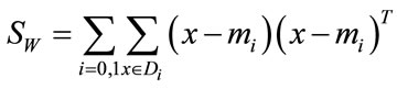
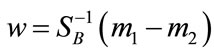
A solution to Equation (3) can be found by solving the generalized eigenvalue problem
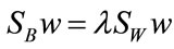
arisen from the decent problem . Since we seek the hyperplane w that optimizes
|
 . Notice that the rank of SW is at most
 , thus care needs to be taken in obtaining a numerically stable and accurate expression for
 . Methods such as regularization and GSVD were proposed to deal with the singularity of SW [8].
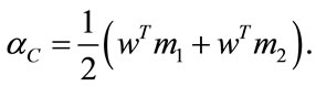
The binary-labeled data is linearly separable if and only if there exists a threshold cutoff value  such that
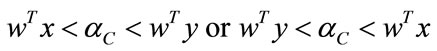
for all  and
and . Without loss of generality, let
 . We let
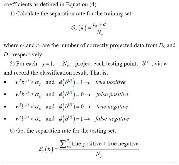

Alternatively, one could define
Accordingly, we define the separation rate of the given data to be
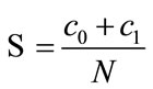
where c0 and c1 are the number of correctly projected data from D0 and D1, respectively.
Due to the small size of our data sets, a leave-one-out cross-validation (LOOCV) is implemented on the UNC data set since not all of the medical features are available on the NYU data set. As the name suggests, this involves using a single observation from the original sample as the validation data, and the remaining observations as the training data. This is repeated such that each observation in the sample is used once as the validation data.
On the other hand, a separation rate that is over 50% is typically not good enough for us to conclude a causaleffect relationship. If a data set of 100 has ten cases that are “At Risk” while the rest are “Not at Risk”, then a separation rate of 50% indicates that the classifier is doing much worse than simply guessing “Not at Risk” all the time which will guarantee a correct answer 90% of the time. Thus, we introduce the Classifier Confidence Rate (CCR) as the level of confidence for a given classifier. As before, let N be the total number of samples in the data set. If each point, xi, in the set is assigned either a label of 0 or 1 under the map , then
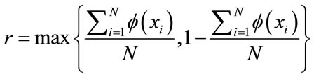
gives the prior statistics. That is, any reliable classifier should perform at least as well as the prior statistics. Then the probability of that classifier with accuracy  produces a non-reliable classification outcome is given by
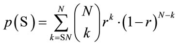
where  gives the number of incidences that are correctly identified. Now, the Classifier Confidence Rate is defined to be the minimum classification accuracy to guarantee a confidence level of
  (e.g.,
  gives a 95% confidence level), i.e.,
Since CCR of a classifier depends on the population statistics, we can use it to gauge the statistical validity of the classification outcomes in the experiments for any particular choice of the data set.
6. Experiments and Results
As mentioned previously, the main driving force in using PCA and LDA is to analyze correlation between shape and medical features, and potentially to predict medical conditions based on placental surface shape alone. Here we will outline the two experiments implemented to accomplish these goals for the UNC and NYU data sets. Recall that the data matrices for each of the data sets  and
and —store the shape information for each placenta. At the same time, the feature information described in Section 2.2 labels each placenta with a 0 or 1, depending on the feature.
6.1. Experiment I
he first experiment isolates one feature at a time, for a total of 16 times, from the UNC data set. After the label ing is established, we implement a Leave-One-Out Cross Validation scheme to produce a separation rate for the UNC data set while varying the number of PC retained. The idea behind this experiment is to exhaustively search for the best separation rate on the data set. A pseudocode for this experiment is given in Algorithm 1 and the resulting best separation rate for each feature label is reported in Table 3.
When the separation rates are compared with their respective classifier confidence rate, which are also found in Table 3, we found that only two feature labels give significant correlational results—BWT Labeling Scheme I
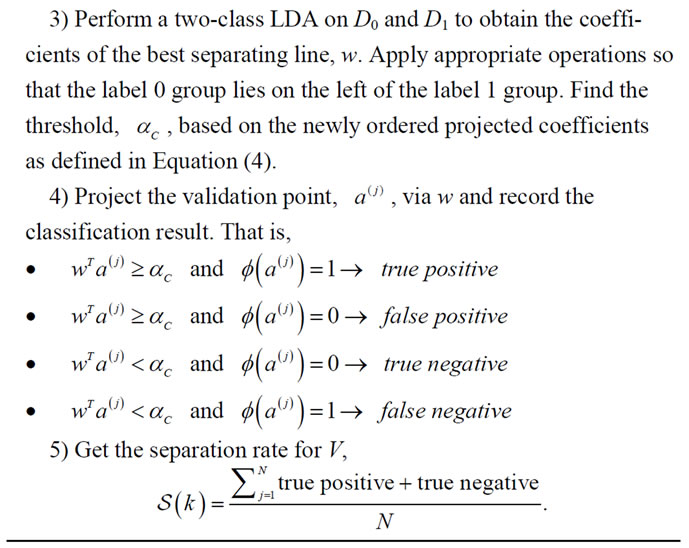

Algorithm 1. LOOCV on UNC.

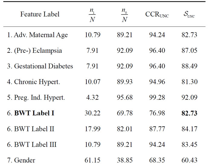
Table 3. The best separation rate (in %) with LOOCV for each feature label in the UNC data set.  and
and  give the percentage of the label 1 and label 0 group in the data set, respectively. CCRUNC gives the classifier confidence rate with 95% confidence level and
  gives the best separation rate obtained while varying the number of PCretained.
and preterm vs. term. A further examination in Figure 11 indicates that the best separation rate is obtained with the first four and five PC for BWT Labeling Scheme I and preterm vs. term, respectively. This confirms the fact that a linear separation cannot be observed when data points are visualized in 2D and 3D, as shown in Figure 9.
Since previous studies have found that placental surface shape is correlated with birth weight when the shape information is described by a scalar measure similar to that of the symmetric difference [5], it is not surprising to see a significant separation rate for the birth weight labeling scheme I in our study. This also confirms with the fact that practicing obstetricians tend to use the Labeling Scheme I as a cutoff for assigning health risks. As shown in Section 4.1, the shape of normality is a round placenta with the umbilical cord centrally inserted, which is consistent with the intuitive concept of optimal blood flow in the vascular network. Deviation from such prototypical shape is shown here to be related to the resulting birth weight.
The feature labeling the gestational age as preterm or
 (a) (b)
Figure 11. Separation rate obtained with LOOCV on the UNC data set while varying the number of PC retained when the feature label is (a) BWT Labeling Scheme I and (b) preterm vs. term.
term also results in a significant separation rate in comparison to the distribution of the set. The medical implications here warrant further investigation since it may be that an irregular placenta shape can cause a preterm delivery, or that other events that cause preterm labor also cause irregular shape. Since we are not making any speculations as to what maternal characteristics causes these listed medical conditions, we can only make an conservative suggestion that placental surface shape alone can be used to make a modest prediction for a child’s birth weight and placental surfaces of termed and pretermed births have noticeably different shape information.
Among the 16 studied features, the gender group has the most balanced data, i.e., the lowest prior statistics. It is not surprising that the gender of the fetus shows no linear correlation with the placental shape. No previous study has shown that the placenta of a male fetus is more or less irregularly shaped than that of a female. The other features, including advanced maternal age, the presence of eclampsia, gestational diabetes, pregnancy induced hypertension, chronic hypertension, inflammation and pathology, did not result in significant separation rates. These results could be explained in the following two ways. Either the variance of these features is not reflected in the geometric placental shape, or these features merely do not give rise to a linear separation due to under-sampling. We remark that while the separation is not perfect with a linear discriminant, a nonlinear classifier derived from methods such as Kernel Discriminant Analysis or Support Vector Machines may suggest a significant result and should be investigated further.
6.2. Experiment II
The second experiment draws the success from Experiment I to test the proposed shape metric as a descriptor to predict health risks based on learned information. LDA classifier is first trained on the UNC data set to learn the class variances and later applied to the NYU data set to obtain classification statistics. The purpose of this set of experiments is to examine the predictive power of the proposed shape descriptor in a realistic setting where no prior information is known for the test set. Assuming the technology allows for an early-stage detection of placental surface shape, medical advices can be given based on the result of this shape analysis.
Recall that the features for the NYU data set are restricted to only birth weight, gender, and gestational age. The shape data with the matching features in the UNC data set are used as the training set for the classification of the new placentas from NYU. After specifying a particular feature, a pseudocode for this experiment is given in Algorithm 2 and the resulting best separation rate for each available feature label is reported in Table 4.
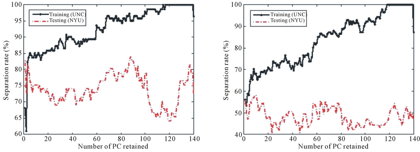
Notice that the NYU data set is populated with more cases of “Not at Risk” under all three labeling schemes and all babies were delivered termed. Except for the case for gender, this test data set poses quite a challenge for the classifier due to this uneven distribution. In the case of gender, assertion can be made that no linear correlation is observed hence indicating the gender of the baby does not influence the shape of the placental surface. Although none of the BWT labels or the Preterm label are associated with a statistically significant result, we suspect that the classifier can be improved given more samples for training and testing as well as the use of non-linear methods for drawing correlation results.Similar to that in Experiment I, a detailed examination of separation rate versus number of PC retained for each feature label is given in Figures 12 and 13 for completion.
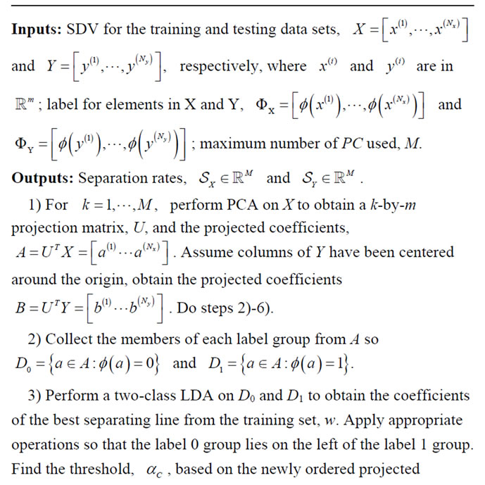
Algorithm 2. Train on UNC, test on NYU.
7. Conclusions
In this study, a near-continuous shape descriptor termed signed deviation vector was proposed as a mathematical representation to capture the deviation of a placental surface away from a prototypical shape. A protocol for automatically registering 2D digital placenta images was described and implemented on the UNC and NYU data sets.
Using Linear Discriminant Analysis (LDA), we independently examined how much of the placental shape is affected by maternal characteristics such as the pregnancy-induced hypertension and medical diagnoses as well as fetal characteristics such as gestational age of the newborns. Experimental results are obtained using a subset
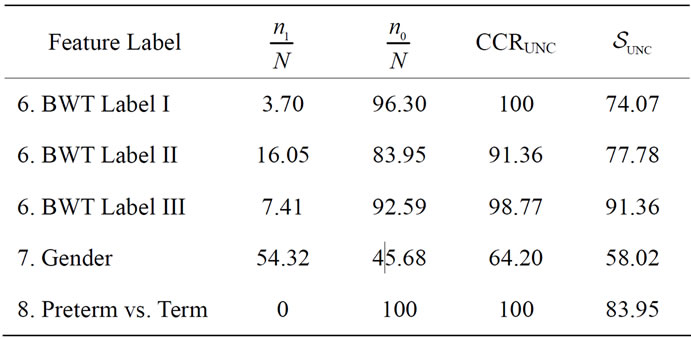
Table 4. The best separation rate (in %) for the available feature labels in the NYU (testing) data sets.  and
and  give the percentage of the label 1 and label 0 group in the data set, respectively. CCRUNC gives the classifier confidence rate with 95% confidence level and
  gives the best separation rate obtained while varying the number of PC retained.
of a birth cohort with 220 ground truth digital images of placental surfaces manually traced by a human expert with a training set of 139 and a testing set of 81. LDA is used to obtain an optimal projection direction using the shape information to achieve the best linear separation on the training set with a Leave-One-Out statistics. When the cases from the testing set are projected accordingly, we are able to draw conclusions from the resulting separation rates as to which medical feature has a significant effect on the shape of placental surface and vice versa. A separation rate that is over the classifier confidence rate is considered a significant result. In these initial findings, we observed suggestive relationship between shape of the placental surfaces and newborn’s birth weight as well as their gestational age. A future study to visually categorize the geometry of placental surfaces that belong to high birth weight and low birth weight groups would be of interest.
There are many possible avenues for continued research in this area. For example, classification algorithms that are nonlinear in nature could be used for making the connection between medical features and shape of the placentas. Other geometric features on the placental surface such as the ones extracted from the placental vasculature network might also offer discriminatory information. The signed deviation vector appears to be a promising measure of deviation from the shape of normality.
While our data sets were only accompanied by limited medical features, we can imagine using the proposed shape descriptor to analyze shape correlation with other medical features that are useful in clinical practice and patient care. For example, it would be interesting to have follow-up information about the health of the children as they grow. What were their APGAR scores that measures immediate health upon delivery? Did they need immediate care in the neonatal intensive care unit, or were they
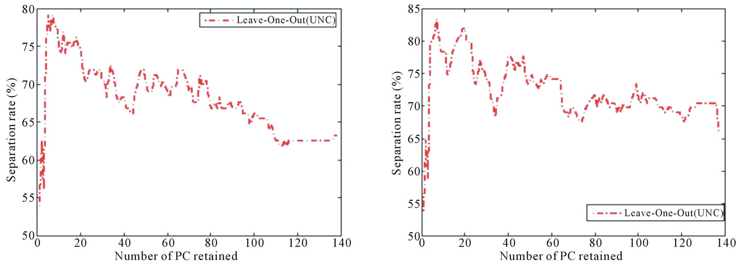
 (a)
(a)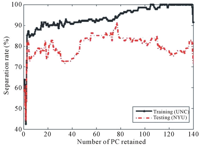 (b)
(b)
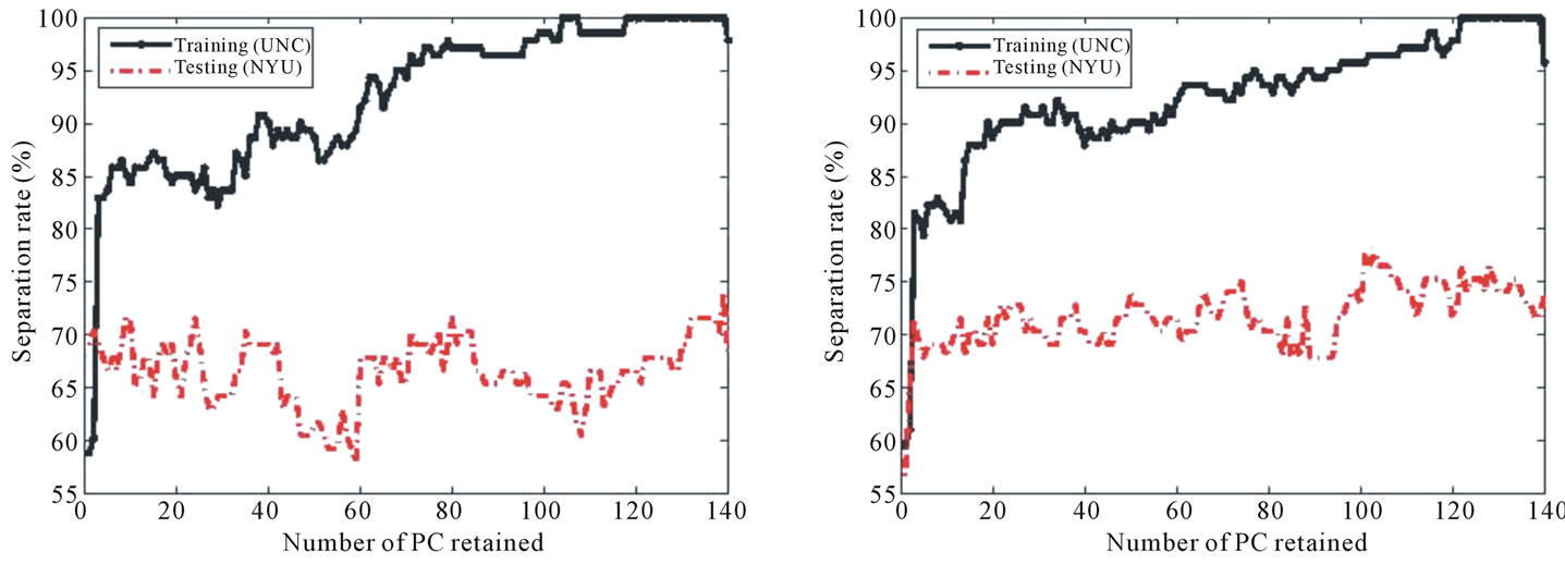
Figure 12. Separation rate for the training (UNC) and testing (NYU) data sets while varying the number of PC retained for (a) BWT Label I, (b) BWT Label II, and (c) BWT Label III. The best separation for each labeling scheme occurs when 139, 101, and 77 PCs are retained for Labeling I, Labeling II, and Labeling III, respectively.
 (a) (b)
Figure 13. Separation rate for the training (UNC) and testing (NYU) data sets while varying the number of PC retained for the (a) preterm vs. term and (b) gender feature label. The best separation rate for the preterm vs. term label occurs when 88 PCs are retained.
discharged soon after delivery? Did they develop a neurodevelopmental disorder, such as developmental delay or an autism spectrum disorder? It could be helpful to use the information immediately available from the placenta after birth to help physicians learn more about a child’s health, and to potentially help with early diagnosis of complicated diseases.
Although our study compares the shape to medical features that are also readily available to physicians, the same methods can be applied in the future to medical features and conditions more difficult to diagnose.
REFERENCES
- M. Yampolsky, C. Salafia, O. Shlakhter, D. Haas, B. Eucker and J. Thorp, “Centrality of the Umbilical Cord Insertion in a Human Placenta Influences the Placental Efficiency,” Placenta, Vol. 30, 2009, pp. 1058-1064. doi:10.1016/j.placenta.2009.10.001
- M. Yampolsky, C. Salafia, O. Shlakhter, D. Haas, B. Eucker and J. Thorp, “Modeling the Variability of Shapes of Human Placenta,” Placenta, Vol. 29, 2008, pp. 790- 797. doi:10.1016/j.placenta.2008.06.005
- D. Savitz, N. Dole, J. Williams, J. Thorp Dr., T. McDonald and C. Carter, “Determinants of Participation in an Epidemiological Study of Preterm Delivery,” Pediatric Perinatology Epidemiology, Vol. 13, 1999, pp. 114-126. doi:10.1046/j.1365-3016.1999.00156.x
- N. Almoussa, B. Dutra, B. Lampe, P. Getreuer, T. Wittman, C. Salafia and L. Vese, “Automated Vasculature Extraction from Placenta Images,” Proceedings of the SPIE Medical Imaging Conference, Florida, February 2011.
- C. Salafia, M. Yampolsky, D. Misra, O. Shlakhter, D. Haas, B. Eucker and J. Thorp, “Placental Surface Shape, Function, and Effects of Maternal and Fetal Vascular Pathology,” Placenta, Vol. 31, 2010, pp. 958-962. doi:10.1016/j.placenta.2010.09.005
- G. Cunningham, “Williams Obstetrics,” McGraw-Hill Publishing, New York, 2005.
- C. Salafia, D. Misra, M. Yampolsky, A. Charles and R. Miller, “Allometric Metabolic Scaling and Fetal and Placental Weight,” Placenta, Vol. 30, 2009, pp. 355-360. doi:10.1016/j.placenta.2009.01.006
- C. Park and H. Park, “A Comparison of Generalized Linear Discriminant Analysis Algorithms,” Pattern Recognition, Vol. 41, 2008, pp. 1083-1097. doi:10.1016/j.patcog.2007.07.022
- M. Wang, A. Perea and R. Gutierrez-Osuna, “Principal Discriminants Analysis for Small-Sample-Size Problems: Application to Chemical Sensing,” IEEE Proceedings of Sensors, 2004, pp. 591-594.
- M. Turk and A. Pentland, “Eigenfaces for Recognition,” Journal of Cognitive Neuroscience, Vol. 3. No. 1, 1991, pp. 71-86. doi:10.1162/jocn.1991.3.1.71
- P. Belhumeur, J. Hespanha and D. Kriegman, “Eigenfaces vs. Fisherfaces: Recognition Using Class Specific Linear Projection,” IEEE Transactions on Pattern Analysis and Machine Intelligence, Vol. 19, 1997, pp. 711-720. doi:10.1109/34.598228
- R. Fisher, “The Use of Multiple Measurements in Taxonomic Problems,” Annals of Eugenics, Vol. 7, 1936, pp. 179-188. doi:10.111/j.1469-1809.1936.tb02137.x.