Applied Mathematics
Vol.4 No.4(2013), Article ID:30357,6 pages DOI:10.4236/am.2013.44083
Fisher’s Fiducial Inference for Parameters of Uniform Distribution
1Society of Old Scientist & Technicians, Xi’an Jiaotong University, Xi’an, China
2College of Information and Computation, National University in the North, Yinchuan, China
3Office of Financial Affairs, Xi’an Jiaotong University, Xi’an, China
Email: wukefa@mail.xjtu.edu.cn
Copyright © 2013 Kefa Wu et al. This is an open access article distributed under the Creative Commons Attribution License, which permits unrestricted use, distribution, and reproduction in any medium, provided the original work is properly cited.
Received June 16, 2012; revised March 12, 2013; accepted March 19, 2013
Keywords: Fiducial Inference; Uniformly Distribution; Parameters; Fiducial Interval; Hypothesis Testing
ABSTRACT
Fisher’s Fiducial Inference for the parameters of a totality uniformly distributed on  is discussed. The corresponding fiducial distributions are derived. The maximum fiducial estimators, fiducial median estimators and fiducial expect estimators of
 ![]() and
and  are got. The problems about the fiducial interval, fiducial region and hypothesis testing are discussed. An example which showed that Neyman-Pearson’s confidence interval has some place to be improved is illustrated. An idea about deriving fiducial distribution is proposed.
1. Introduction
In 1930 Fisher proposed an inference method based on the idea of fiducial probability [1,2]. Fisher’s fiducial inference has been much applied in practice. The fiducial argument stands out somewhat of an enigma in classical statistics. The enigma mentioned above need statistical scholar to solve.
Fisher’s fiducial inference for the parameters of a totality  is discussed. The corresponding fiducial distributions are derived. The maximum fiducial estimators, the fiducial median estimators and the fiducial expect estimators of
 ![]() and
and  are got. The problems about the fiducial interval, fiducial region and hypothesis testing are discussed.
The example below shows that Neyman-Pearson’s confidence interval has some place to be improved. Let  be i.i.d.,
  for each j.
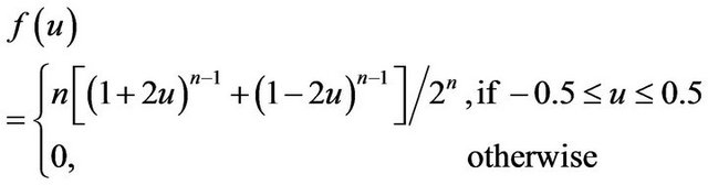
 . By [3] p. 16 Corollary 3.2 the density function of
  is
is

Appling pivotal function
And using its density
the 95% confidence interval of  can be got as
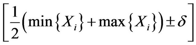 (*)
(*)
where ![]() is the solution of
is the solution of
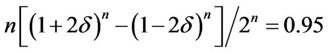
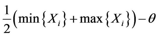
The length of interval (*) is independent of the sample value! Assam that
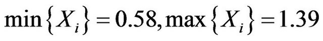
Is got in a certain sample (Note that
 the above data can illustrate the common problems). The probability that
i.e.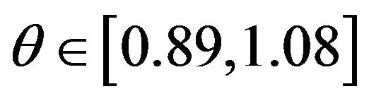 , is 1, the length of it is 0.19, but the length of (*) is
Fisher’s fiducial inference offered a selection in solving the problems similar with above.
2. Fiducial Distribution
Let that  is i.i.d.,
 . As well known, their sufficient statistics of least dimension is
 .Set
.Set
 (2.1)
(2.1)
It is not difficult to show that Y and Z are the minimum and maximum order statistics of the sample from  respectively, and by [3] p. 16 Corollary 3.2, the density function of
  is
is
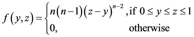 (2.2)
(2.2)
See parameters ![]() and
and  as r.v.’s, see
  and
and  as constants now. It can be got from Equation (2.1) that
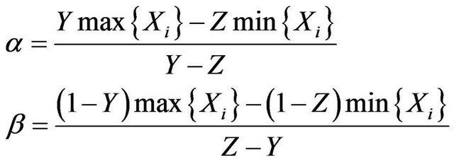 (2.3)
(2.3)
Applying the relative results about the transformation of r.v.’s, it can be show that:
Theorem 1. The fiducial density function of vector  is
is
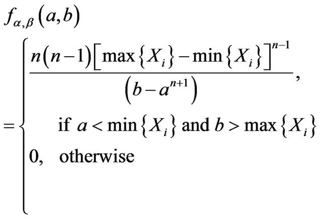 (2.4)
(2.4)
If only one parameter need to be considered, the another parameter is then so-called nuisance parameter. We insist that the marginal distribution should be used in this situation. Hence find the two marginal density functions of 
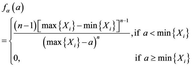 (2.5)
(2.5)
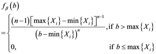 (2.6)
(2.6)
Corollary 1. The fiducial density functions of only one parameters ![]() or
or  as r.v.’s are given by (2.5) and (2.6).
3. Estimation
It is easy to see that fiducial density  has achieved its maxima at
 (3.1)
(3.1)
 (3.2)
(3.2)
Theorem 2. The maximum fiducial estimators of ![]() and
and  are given by (3.1) and (3.2).
It can also be got that  has achieved its maxima at
 , and
, and  has achieved its maxima at
  as well. The estimators
  and
and  are coincided with the maximum likelihood estimators of
 ![]() and
and .
.
To find the median of , solve
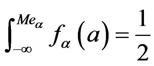 (3.3)
(3.3)
And get
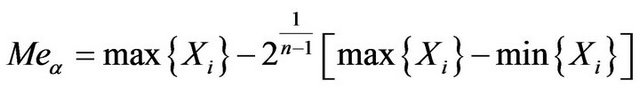 (3.4)
(3.4)
Found the median of  by using the same method, and have
 (3.5)
(3.5)
Theorem 3. The fiducial median estimators of ![]() and
and  are given by (3.4) and (3.5).
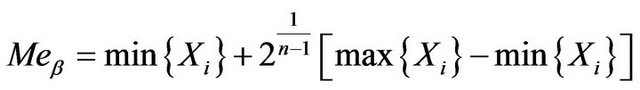
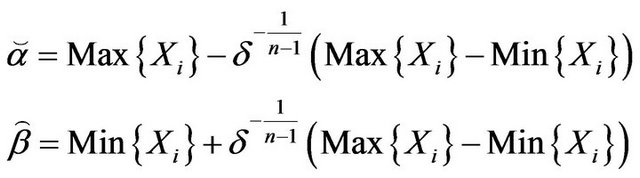
The maximum fiducial estimators  and
and  are extreme a little, Equation (3.1) can be written as
Since
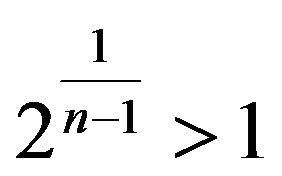
 is a modify to
 , and
, and  is a modify to
  too.
too.
It can be shown that:
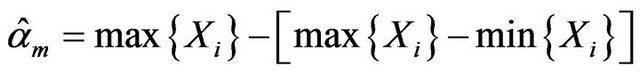
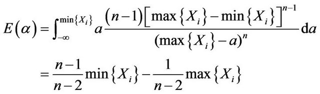
Theorem 4. The fiducial expect estimators of ![]() and
and  are given by
 (3.6)
(3.6)
wang#title3_4:spProof.
 can be calculated by using the same method. □
 is a better modify to
 , and
, and  is a better modify to
  as well. We suggest using
  and
and .
.
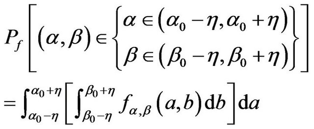
The fiducial probability that ![]() belongs to a certain interval estimator
belongs to a certain interval estimator  can be calculated using
  as follows
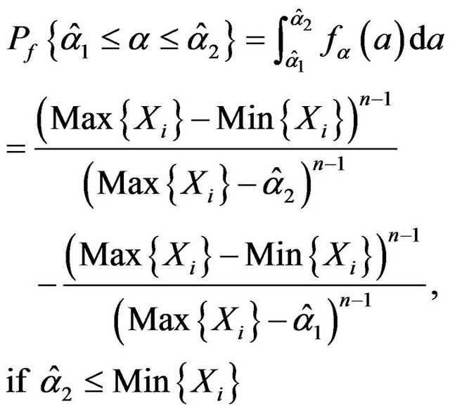 (3.7)
(3.7)
In the same way
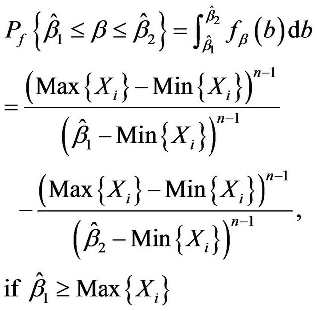 (3.8)
(3.8)
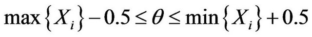
Give a fiducial probability  let us consider the
  fiducial interval problem. In order to set the length of the interval as shorter as possible, we choice
  as the right end point of the fiducial interval of
![]() , because
, because  increases; and choice
  as the left end point of the fiducial interval of
 , because
  decreases.
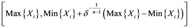
Theorem 5. The  fiducial interval of
 ![]() is
is
 (3.9)
(3.9)
The  fiducial interval of
  is
is
 (3.10)
Proof. Denote that
Using (3.7) it can be derived that
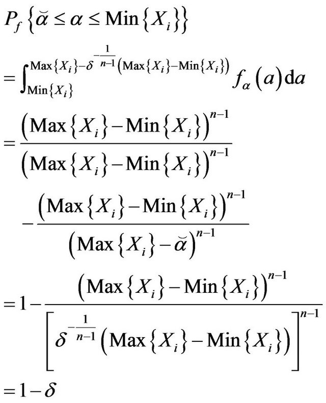
And the bellow equation can be got by using (3.8)
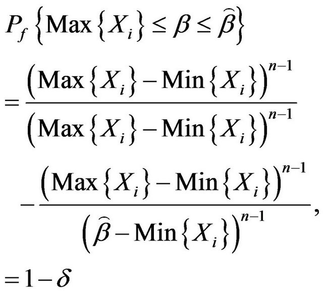 □
□
Let us consider the  fiducial region of
 . In order to set the area of the region as smaller as possible, we choice the region as the following rectangular triangle:
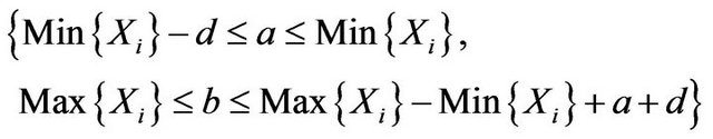 (3.11)
for a certain d > 0, because  choice the same value when
  equals to a constant, and
  increases in a when b is invariant, decreases in b when a is invariant.
Theorem 6. The  fiducial region of
  is given by (3.11) if positive d satisfies
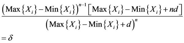 (3.12)
Proof. At first Equation (3.12) has a positive solution d because its left side equal to 1 when  and tends to 0 when d tends to
![]() . Hence the fiducial probability that
. Hence the fiducial probability that  belongs to the region given by (3.11) is
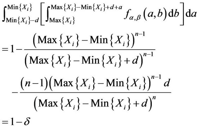
Equation (3.12) is used here. □
4. The Case That One Parameter Is in Variation
Let us consider the case that only one parameter is in variation.
 is a distribution with single-parameter when one end point of
  is constant. For constant b0
 is sufficient for
 . It can be got that the fiducial density of parameter
 ![]() in
in  is
is
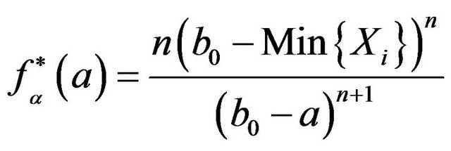 (4.1)
(4.1)
It should noted that using (2.4) and (2.6) the conditional density of ![]() under
under  can be got as
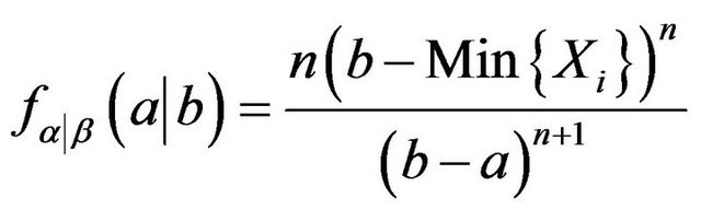 (4.2)
(4.2)
Comparing (4.1) and (4.2) is to say that (4.1) is coincided with the conditional density of ![]() under
under 
The maximum fiducial estimators, the fiducial median estimators and the fiducial expect estimators of ![]() can be got easily by using (4.1).
can be got easily by using (4.1).
The fiducial probability of one interval estimator  for
for ![]() can be calculated as
can be calculated as
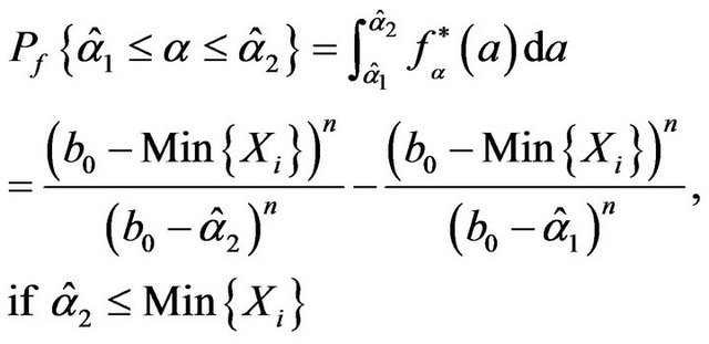 (4.3)
(4.3)
The  fiducial interval of
 ![]() can be got as follows by using (4.3).
can be got as follows by using (4.3).
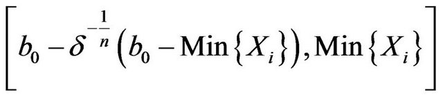 (4.4)
(4.4)
The similar results for  can be got easily as well.
If there is a relation between the parameters, such as the example in Section 1, this situation may be thought as missing parameter(s). We insist that the conditional distribution should be used in this situation. Under the condition that  for a constant C, the conditional density
 , or
, or![]() , is a constant in the interval on which its value isn’t zero, because
, is a constant in the interval on which its value isn’t zero, because  is a constant when
 . Since
 the conditional density
  is the density of
 . This is the fiducial density of the parameter
 ![]() of a totality
of a totality .
.
It can be seen that for distribution ,
,

is a 100% fiducial interval of![]() . Any subinterval of
. Any subinterval of
is a  fiducial interval of
 ![]() in this problem only if it has the length
in this problem only if it has the length
 .
.
Using the above results to the example in Section 1 it can be got that any subinterval of [0.89, 1.08] with the length 0.95 × 0.19 is the 95% fiducial interval of . Its length 0.1805 is much smaller than
 , the length of interval (*).
5. Hypothesis Testing
Let us consider the hypothesis testing problem. Equation (3.7) and (3.8) can be used to calculate the fiducial probability when the parameter would belong to the range that a certain hypothesis is true.
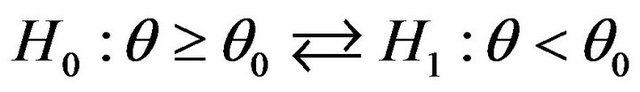
Theorem 7. For hypothesis
 (5.1)
(5.1)
And should rejected H1 w.p.1 if .
.
Proof. Choice  and
and  in (3.7). □
If for a certain , the decision is made by comparing
  with
with , then the criterion is that reject H0 when
 (5.2)
(5.2)
Note that the left hand of (5.2) is the quantile of order
 of the fiducial distribution of
![]() . Especially for
. Especially for
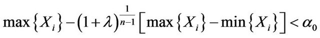
 the criterion is reject H0 when
 (5.3)
(5.3)
Theorem 8. For hypothesis
The fiducial probability

Proof. The result can be got just like theorem 7. □
The parallel results for  can be got by using the same method as well.
Theorem 9. Hypothesis
The fiducial probability
wang#title3_4:spProof.
This theorem can be got by calculating the above integral. □
The fiducial probability in the situation that the parameters would belong to the range that a certain hypothesis in Theorem 7 or 8 is true can be easily got by using (4.3) in the case that one parameter is in variation.
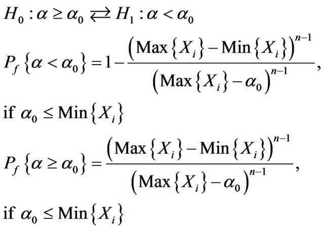
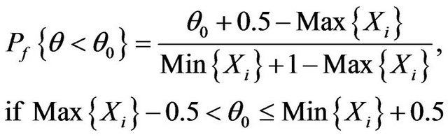
Example. For the example in Section 1, consider the hypothesis
It can be shown that
If for a certain , the decision is made by comparing
  with
with , when the one in front is greater,
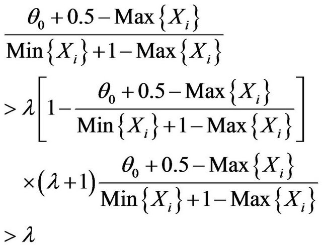
So the criterion is that reject H0 when
 (5.4)
(5.4)
Please note that the left hand of (5.4) is the quantile of order  of the fiducial distribution of
 . Especially for
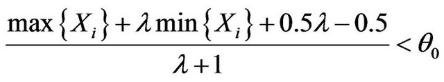
  the criterion is that reject H0 when
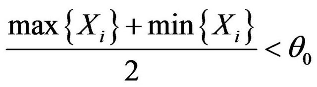 (5.5)
(5.5)
That is
 (5.6)
(5.6)
6. Discussion
Up to now, the discussion on Fisher’s fiducial inference has still remained intuitive and imprecise. There are two problems: 1) Just what a fiducial probability means? 2) How can one derive the only fiducial distribution of the parameter(s)? Paper [4] considered the 1st problem. For the 2nd problem we guess that two sufficient statistics of least dimension, whose dimension is coincides with the parameter(s), must derive the same fiducial distribution of the parameter(s). And we insist that the marginal distribution should be used in the situation when there is (are) nuisance parameter(s); and that the conditional distribution should be used in the situation when there is (are) (a) relation(s) between the parameters.
REFERENCES
- R. A. Fisher, “Inverse Probability,” Proceedings of the Cambridge Philosophical Society, Vol. 26, 1930, pp. 528- 535.
- S. L. Zabell, “R. A. Fisher and the Fiducial Argument,” Statistical Science, Vol. 7, No. 3, 1992, pp. 369-387. doi:10.1214/ss/1177011233
- J. C. Fan and K. F. Wu, “A Introduction of Statistical Inference,” Science Press, Beijing, 2001.
- K. F. Wu, “The Relativity of Randomness and Fisher’s Fiducial Inference,” The 4th ICSA Statistical Conference, 1998, Kunming, Abstracts #88.