Modern Economy
Vol.06 No.05(2015), Article ID:56322,14 pages
10.4236/me.2015.65051
Recommended Methods to Re-Calculate Regional and Total Economic Surpluses after Solving Spatial Equilibrium Models by the Non-Linear Programming Method
Phan Sy Hieu1, Steve Harrison2,3, Dominic Smith4
1Center for Informatics and Statistics, Ministry of Agriculture and Rural Development, Hanoi, Vietnam
2School of Economics, the University of Queensland, Brisbane, Australia
3School of Economics, the University of the Sunshine Coast, Sunshine Coast, Australia
4Helvetas Organization, Hanoi, Vietnam
Email: hieu_ps@yahoo.com, s.harrison@uq.edu.au, Dominic.Smith@helvetas.org
Copyright © 2015 by authors and Scientific Research Publishing Inc.
This work is licensed under the Creative Commons Attribution International License (CC BY).
http://creativecommons.org/licenses/by/4.0/


Received 2 February 2015; accepted 12 May 2015; published 14 May 2015
ABSTRACT
The current non-linear programming method does not derive regional economic surpluses and may derive an imprecise maximized value of the total economic surplus. The main reason is that the integrals for supply functions will automatically take regional non-economic producer surpluses into account if any intercepts of supply functions is negative. Consequently, the derived va- lues are always lower than the real regional and total economic surpluses. The unknown regional economic surpluses and the imprecise total economic surplus will limit the suitable application of the model for broader contexts including game theory analysis, international trade policy analysis, and even GDP calculation. This paper recommends two formulae applied for two types of functions, namely original and inverse supply and demand functions, to calculate the regional and total economic surpluses of commodities. The two methods can be converted to each other conveniently, for example by using an inverse matrix of coefficients of original supply and demand functions to solve coefficients of inverse supply and demand functions. A numerical example is used to illustrate the spatial equilibrium model for 2 products and 3 regions with original linear supply and demand functions.
Keywords:
Producer Surplus, Consumer Surplus, Negative Intercepts, Integrals of Supply and Demand

1. Introduction
The concept of the spatial equilibrium model was raised in the late 19th century [1] . The mathematics of the model have undergone step by step developed since 1950. The mathematical model was developed firstly by Enke in 1951 and independently by Samuelson in 1952. Samuelson was the first person who stated that the spatial equilibrium between various markets might be solved by mathematical programming, and formulated the problem as the maximization of the area under all excess demand curves, plus the area under all excess supply curves, minus the total transportation costs [2] . Later, the spatial equilibrium model with the quadratic objective function was developed partially by Takayama and Judge in 1964 and fully by these authors in 1973 [1] .
Until 2011, there were three common methods applied to derive optimal solutions for spatial equilibrium models. Non-linear programming is the most common method used to solve spatial equilibrium models with a non-linear objective function for the total economic surplus including linear and non-linear supply and demand functions as presented in journal articles and mathematical programming books including Takayama and Judge (1964) [3] and McCarl and Spreen (2002) [4] .
Linear programming is used to solve spatial equilibrium models with linear supply functions, linear demand functions, and linear objective function of the total transportation cost as presented in Phan, Harrison, and Lamb (2011) [5] . Mixed complementary programming is used to derive optimal solutions for spatial equilibrium models without any objective function, as presented in Goletti et al. (1996) [6] , but requires some strict conditions and in particular equal numbers of constraints and equations [4] . All three methods were published on the website of the General Algebraic Modeling System (GAMS) in November 2010 as presented in Phan (2010) [7] . Various software packages can be used for the three programming methods, for example the Solver facility in Microsoft Excel (for relatively small models) and the General Algebraic Modeling System (GAMS) software which will solve models with tens of thousands of activities and constraints [1] .
Spatial equilibrium models have been applied for some commodities in some countries since the 1970s, for example, Hall, Heady, Stoecker, and Sposito (1975) [8] for agriculture in the USA, Uri (1975) [9] for electrical energy in the USA, Jae (1984) [10] for southern pine lumber in the USA, Goletti et al. (1996) [6] for the rice sector in Vietnam, Tsunemasa, Nobuhiro, and Harry (1997) [11] for an imperfect milk market in Japan, ACI (Agriculture Consultant International) (2002) [12] for the livestock sector in Vietnam, Stennes and Wilson (2005) [13] for lumber markets in the USA and Canada, Devadoss, Angel, Steven, and Jim (2005) [14] for softwood lumber markets in the USA, Canada, Mexico, China, Japan, New Zealand, Australia and the European Union, Betty, Nelio, and Andres (2010) [2] for soybean production in Tocantins and neighboring states in Brazil, Phan, Harrison and Lamb (2011) [5] for wood-processing products in northern Vietnam, Shu-ichi and Nobuhiro (2011) [15] for Japan’s electric power network, Seyed and Abdoulkarim (2012) [16] for rice products in Iran, Paul, David, and Benjamin (2014) [17] for unemployment and wage bargaining, and Yanjie, John, Alicia, Ying, and Fei (2015) [18] for global wood products.
In terms of economic-reality aspects, the three methods can derive correctly optimal solutions of regional prices, regional supply quantities, regional demand quantities, regional transport quantities, and the total trans- portation cost. However, the optimal solution derived for the total economic surplus can be imprecise. In addi- tion, the current methods do not calculate regional economic surpluses in aggregate or for each specific commo- dity. Therefore, the following sections examine why the two limitations exist and proposes how to solve preci- sely the economic surpluses of commodities, regional economic surpluses, and the total economic surplus gene- rated by the spatial equilibrium models with linear supply and demand functions.
2. The Operation of a Simple Theoretical Spatial Equilibrium Model
The spatial equilibrium model is the broadest market equilibrium model [1] . The spatial equilibrium model determines the equilibrium prices and quantities simultaneously, not only in all markets but also in all regions. Figure 1 describes how a simple spatial equilibrium model for one product and two regions moves to the optimal point.
When the commodity can be traded between two regions, the commodity is transported from a lower price region to a higher price region―from Region 1 to Region 2 in Figure 1. When producers in Region 1 transport their product to Region 2, the price in Region 1 increases and the price in Region 2 falls. The price difference between the two regions is reduced until it is less than or equal to the unit transportation cost [1] . If applied to the same region for different products and zero unit transportation cost, the model becomes a general equili-
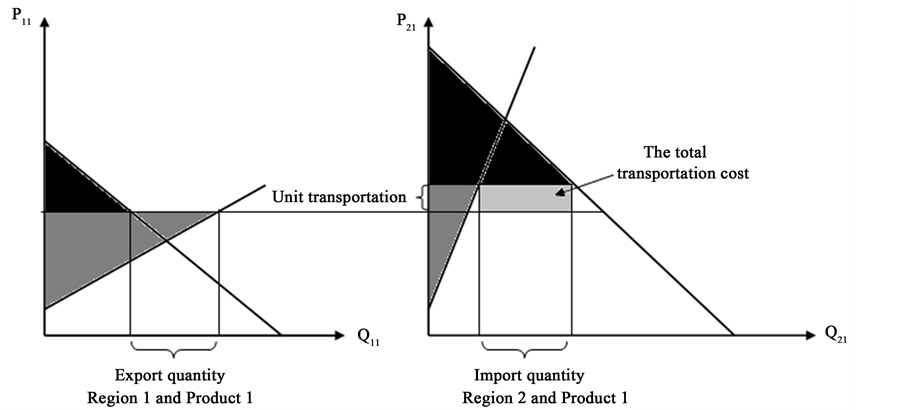
Figure 1. Regional consumer and producer surpluses of a simple theoretical spatial equilibrium model for 1 product and 2 regions.
brium model. And, if the unit transportation cost is higher than the price difference between regions, the two regions are separated and this simple model can be split into two partial equilibrium models [1] .
For a general case―a spatial equilibrium model for multiple products and multiple regions―the theoretical explanation for the commodity movement is that “the quantity traded is the amount such that the total economic surplus of all products of all regions is maximized” or “the quantity traded is the amount such that the total transportation cost of all products between all regions is minimized”. Mathematically, the maximization process leads to the optimal regional prices, regional supply quantities and regional demand quantities, and total economic surplus. The minimization process identifies the optimal quantities traded between regions and the total transportation cost.
In Figure 1, the black triangles for Regions 1 and 2 are the optimal consumer surpluses, the grey triangles for Regions 1 and 2 are the optimal producer surpluses, and the light grey square in Region 2 is the minimized total transportation cost. The sum of optimal consumer surpluses plus the sum of optimal producer surpluses is the maximized total economic surplus. At the optimal or equilibrium status, the export quantity of Region 1 equals the import quantity of Region 2. The import value of Region 2 equals to the export value of Region 1 plus the total transportation cost. The price difference between the two regions is smaller than or equal to the unit transportation cost.
3. Regional and Total Economic Surpluses of a Simple Theoretical Spatial Equilibrium Model with Inverse Linear Supply and Demand Functions
Mathematically, the behavior of producers is expressed as the supply quantity being a function of supply price,
 , called the original supply function. Similarly, the behavior of producers is expressed as the supply price being a function of supply quantity,
 , called the inverse supply function. Similarly, the behavior of buyers can be expressed in two alternative ways,
 or
or . The inverse functions
 and
and
 are applied in most economics and mathematical programming textbooks and international journals, for instance in the economics book by Mansfield (1996) [19] , and in the journal articles of Stennes and Wilson (2005) [13] and Devadoss, Angel, Steven and Jim (2005) [14] . The main reason may be that the application of inverse supply and demand functions in economics textbooks can explain main ideas of economics in an easy-to-understand way, for example illustrating that the total area under the demand curve and above the market equilibrium price line forms the consumer economic surplus.
In almost economics textbooks, the total economic surplus is calculated as the sum of the areas of black and grey triangles presented in Figure 1 by the basic formula to calculate the area of a triangle, as base multiplied by height and then divided by 2. However, in almost programming books, in order to derive conveniently the total economic surplus for large-scale spatial equilibrium models with various types of functions, researchers normally use the integrals of inverse supply and demand functions, representing the areas under the demand curves and areas under the supply curves to calculate the total economic surplus. At an aggregate level, the objective function of the total economic surplus is expressed as the sum of all regional economic surpluses of all com-
modities minus the total transportation cost or . The most currently applied mathe-
matical expression for the simple two-region model is presented below.
Maximize the total economic surplus:

Subject to:


Here:
 : Region
 and region

 : Demand price in region

 : Supply price in region

TE: The total economic surplus
 : Demand quantity in region

 : Supply quantity in region

 : Quantity transported from region
 (export region) to region
 (import region)
 : Unit transportation cost to transport one unit of commodity from region
 to region

In Figure 2, this expression means:
the total economic surplus of the two regions = the black areas in Regions 1 and 2
+ grey areas in Regions 1 and 2
− the light grey area in Region 1
+ the light grey area in Region 2
− the light grey square in Region 2 (the total transportation cost area).
The outcome of the expression presented in Figure 2 is correct or consistent with the theoretical explanation presented in Figure 1 in Section 1. In Figure 2, Part (3) is the result of Part (1) minus Part (2). In Part (3), the total economic surplus will be the sum of all black and grey areas for the two regions. The export quantity of Region 1 equals to the import quantity of Region 2. The import value of Region 2 equals to the export value of Region 1 plus the total transportation cost. The price difference between the two regions is smaller than the unit transportation cost between the two regions. However, this application of integrals will face the two following
difficulties. Unlike at aggregate level, at regional level the similar objective function expressed as ( −
−
the regional transportation cost) does not represent the economic surplus of a region. For example, in the export
region (Region 1), the calculation of ( − the regional transportation cost) represents the black train-
gle area (consumer surplus) plus the grey area (only part of producer surplus) minus the light grey area (the export cost). This implies that if researchers would like to know the regional economic surplus of Region 1, they should plus the total export value but not minus the regional transportation cost, or they should apply the formu-
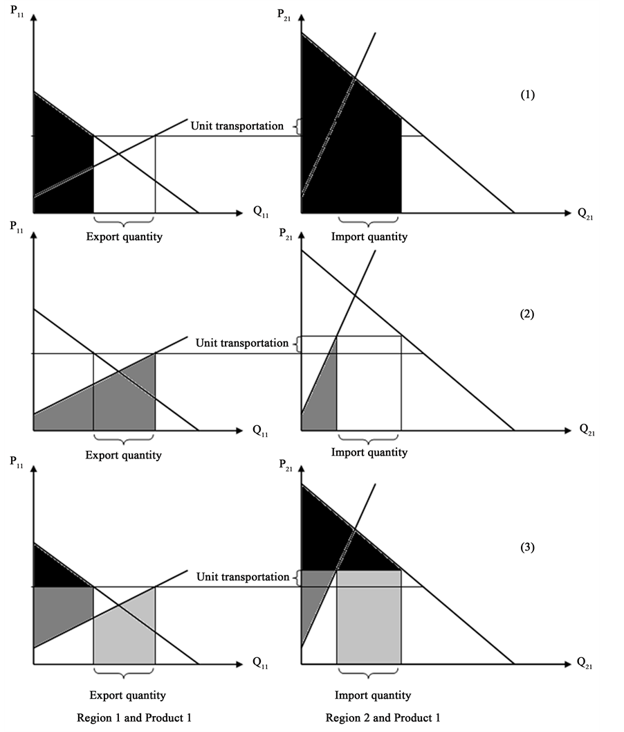
Figure 2. Regional economic surpluses expressed by the application of integrals of inverse linear supply and demand functions with positive intercepts of inverse supply functions.
la:
 + Regional export value.
In the import region (Region 2), the calculation of ( − the regional transportation cost) also does
not present the economic surplus of a region. This calculation represents the black triangle area (consumer surplus) plus the grey triangle area (producer surplus) plus the light grey square area. The light grey square means the import value includes the regional transportation cost. This implies that if researchers would like to know the regional economic surplus of Region 2, they should minus the total import value but not minus the regional
transportation cost or apply the formula:
 − Regional import value.
According to the above formulae, the regional economic surplus of the export or import region does not take into account the regional transportation costs because the regional transportation cost is already included in the regional import values generated automatically by the application of integrals of inverse supply and demand functions. In addition, the current calculation of the total economic surplus by applying the integrals will not be precise if intercepts of any regional inverse supply functions are negative, as presented in Figure 3.
When the intercepts1 of regional supply functions are negative, integrals of regional inverse supply functions will automatically include regional negative non-economic values2 in producer costs, and will reduce the producer surpluses, regional economic surpluses and total economic surplus. The reduced surplus is the area of the
black triangle
 in Figure 3. This situation commonly happens3, so in order to solve the regional and
total economic surpluses correctly, researchers should take into account the case having negative intercepts of inverse supply functions. The recommended formula to re-calculate regional and total economic surpluses for the simple model having negative intercepts of the supply functions is presented below.


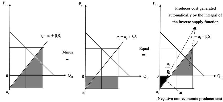
Figure 3. The negative non-economic value is included automatically in the producer cost when the integral calculations are applied for negative intercepts of inverse supply functions .
.
Here:
 : The total economic surplus
 : The economic surplus of region

 : Regional demand quantity, supply quantity at market equilibrium points
 : Regional demand function of
 and regional supply function of

 : Quantity export from region
 to region
 at market equilibrium points
 : Quantity import from region
 to region
 at market equilibrium points
 : The negative intercepts of inverse supply functions in region

 : The positive own-quantity coefficient of inverse supply functions in region

For greater clarity, the recommended formula to re-calculate the regional and total economic surpluses after solving the simple spatial equilibrium model having negative intercepts of the supply functions by the current non-linear programming method is illustrated by six steps in Figure 4.
4. Regional and Total Economic Surpluses of a Simple Theoretical Spatial Equilibrium Model with Original Linear Supply and Demand Functions
Although the coefficients between original and inverse functions can be converted rather conveniently4, fewer studies have used spatial equilibrium models with inverse supply and demand functions than that with original supply and demand functions,
 and
and . The main reason may be that econometric models with original functions are normally used to estimate price coefficients and price elasticities of supply and demand.
Phan and Harrison (2011) [1] found that the application of the objective function of
 or
or
 generates similar optimal solutions of regional supply quantities, regional demand
quantities, regional transport quantities, regional prices, and total transportation cost. However, the solutions differ in terms of how values of objective functions are interpreted. If the objective function of original functions
 is used, the optimal objective value is the total economic cost (producer cost plus
consumer cost), not the total economic surplus as presented in Sections 1 and 25.
Similar to the application of integrals for inverse linear supply functions, the application for original linear supply functions also generates an imprecise regional producer surplus if intercepts of these functions are negative. In addition, the objective function of the total economic cost cannot be used to calculate directly the total economic surplus. Therefore, the five steps listed below set out how to calculate the precise regional and total economic surpluses for studies applying spatial equilibrium models with original linear supply and demand functions.

Figure 4. Steps to re-calculate the regional and total economic surpluses for the simple spatial equilibrium model if intercepts of inverse linear supply functions are negative. Note: the calculation including plus (+) and minus (−) presented in this figure is applied for positive areas of grey shapes.
1. The current method, for example the non-linear programming method with the objective function of , is used to derive the optimal solutions of regional supply quantities, regional demand quantities, regional transport quantities, regional prices, and total transportation cost. The mathematical expression for this simple model is presented below.
Minimize the total economic cost:

subject to:


where:
 : Region i and region

 : Demand price in region i
 : Supply price in region i
TEC: Total economic cost
 : Demand quantity in region i
 : Supply quantity in region i
 : Quantity transported (or exported) from region i to region

 : Unit transportation cost to transport one unit of commodity from region i to region

2. The optimal solutions found in Step 1 are used to calculate the intercepts of the regional original linear demand and supply functions. The formulae to calculate the intercepts are presented below.
For supply functions:

For demand functions:

where:
 : The intercepts of original supply functions in region

 : The positive own-prices coefficient of original supply functions in region

 : The intercepts of original demand functions in region

 : The negative own-price coefficients of original demand functions in region

 : Regional demand quantity, supply quantity at equilibrium points
 : Regional demand price and supply price at equilibrium points.
3. The calculated intercepts of regional original demand functions in Step 2 and the given demand own-price coefficients,
 and
and
 respectively, are used to calculate the whole area under it. The whole area is the total consumer surplus if product price is zero. The recommended formula to calculate the whole areas is:

where:
 : The total value of the whole area under the demand curve of the region

 : The demand quantity and demand price, and
 is a function of
 with found intercepts in Step 1 and given own-price coefficients.
4. If the regional supply intercepts are positive, the regional and total economic surpluses can be calculated by the recommended formulae below:


where:
TE: The total economic surplus
 : The economic surplus of region

 : The total value of the whole area under the demand curve of the region

 : Regional demand price and supply price at equilibrium points
 : Regional demand function of
 and regional supply function of
 respectively.
5. If the regional supply intercepts are negative, the above regional economic surpluses should be adjusted due to the negative non-economic values of producer surpluses generated automatically by the application of integrals of original linear supply and demand functions. The sum of found regional economic surpluses is the precise total economic surplus. The following are recommended formulae to re-calculate regional and total economic surpluses.


where:
 : The negative intercepts of original supply functions in region

 : The positive own-price coefficient of original supply functions in region

For greater clarity, Figure 5 describes steps to calculate precise regional and total economic surpluses for the simple spatial equilibrium model with original linear supply function having negative intercepts and demand functions after the optimal solutions of regional supply quantities, regional demand quantities, regional transport quantities, and regional prices are obtained by the current non-linear programming method.
5. A numerical Example for a Representative Spatial Equilibrium Model with Original Linear Supply and Demand Functions
A numerical example slightly modified from that of Takayama and Judge (1964) [3] is used to illustrate the method of calculating regional and total economic surpluses for the spatial equilibrium model with original linear supply and demand functions. The example having 2 products and 3 regions is fully representative of any spatial equilibrium models with n products and m regions. The hypothetical original linear supply and demand functions for two products in three regions are presented in Table 16.
The unit transportation costs (ti,rr’, the cost to transport one unit of product i from region r to region ) are as in Table 2. For example, the unit transportation cost for product 1 from region 2 to region 1 is 2, and from region 2 to region 3 is 1.
Suppose that an economist would like to find answers for the following 9 questions:
1. What are the optimal regional prices (supply price,
 , equal to demand price,
 )?
)?
2. What are optimal regional supply quantities ?
?
3. What are optimal regional demand quantities ?
?
4. What are optimal regional transport quantities , and import and export values (
 and
and )?
)?
5. What is the minimized total transportation cost (TC)?
6. What are the optimal regional transportation costs ?
?
7. What are the regional economic surpluses and the maximized total economic surplus without taking import and export values and signs of intercepts of supply functions into account (imprecise TE)?
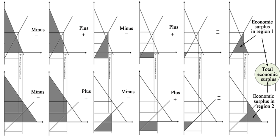
Figure 5. Steps to re-calculate the regional and total economic surpluses for the simple spatial equilibrium models if intercepts of regional original linear supply functions are negative. Note: the calculation including plus (+) and minus (−) presented in this figure is applied for positive areas of grey shapes.

Table 1. Original linear supply and demand functions for two products in three regions.
Note: D is demand quantity, S is supply quantity, pd is demand price, ps is supply price, r is the subscript for region (r = 1, 2, 3) and i is the subscript for product (i = 1, 2).
Table 2. Unit transportation cost between regions.
8. What is the maximized total economic surplus when taking signs of intercepts of supply functions into account (precise TE)?
9. What are optimal regional economic surpluses (precise ), and regional producer surpluses (precise
 ) and regional consumer surpluses (precise
 )?
)?
A non-linear programming model written in a GAMS file with non-linear CONOPT Solver facilities is used to solve for regional prices, regional supply quantities, regional demand quantities, quantities traded between regions, and regional import and export values, as presented in Table 3 and Table 4, in answer to Questions 1 to 47.
The optimal solutions in Table 3 indicate the regional prices of commodity 1 are 11, 9 and 10 in Regions 1, 2 and 3 respectively. Those of commodity 2 are 11.64, 8.64 and 10.64 in Regions 1, 2 and 3 respectively.
Table 3 indicates the regional demand quantities of commodity 1 are 101, 64, and 90 in Regions 1, 2 and 3 respectively. Those of commodity 2 are 195.27, 35.91, and 154.27 in Regions 1, 2 and 3 respectively.
Table 3 indicates the regional supply quantities of commodity 1 are 65.5, 134.5, and 55 in Regions 1, 2 and 3 respectively. Those of commodity 2 are 120.36, 160.23, and 104.86 in Regions 1, 2 and 3 respectively.
Table 3. Optimal solutions of regional prices, regional supply quantities, and regional demand quantities―output of the computer program.
Table 4. Optimal solutions of quantities transported between regions, regional import and export values, as generated by GAMS.
Note: Com. 1 means commodity 1; Com. 2 means commodity 2.
Table 3 indicates that Region 2 is the only surplus region. The supply quantities of the commodity 1 (134.50) and the commodity 2 (160.23) are much higher than the demand quantities of the commodity 1 (64.00) and the commodity 2 (35.91).
Table 4 indicates that the export quantities of Region 2 for commodity 1 of 35.50 to Region 1 and of 35.00 to Region 3. Region 2’s export quantities of commodity 2 are 74.91 to Region 1 and 49.41 to Region 3.
Table 4 indicates that the total import value of Region 1 is 1262.2, and that of Region 3 is 875.5. The total import value of the two regions is 2137.7, and the total export value of Region 2 is 1708.2. The difference between the total export and import values is the total transportation cost paid by consumers in import regions. Solutions by GAMS produces the regional and total transportation costs presented in Table 5, answering Questions 5 and 6.
Table 5 indicates that the regional transportation costs are paid by consumers of the import regions, namely Regions 1 and 3. Region 1 imports greater quantities than Region 3, and with given unit transportation costs, Region 1 pays more transportation cost (295.7) than Region 3 (133.8). The total transportation cost is 429.5. Region 2, the export region, does not pay for transportation costs. The regional transportation costs in Table 5 plus regional export values in Table 4 equal to the regional import values in Table 4.
If an economist does not take into account signs of the intercepts of original linear supply functions, and values of regional imports and exports, the imprecise total economic surplus generated by the GAMS programming is 6224.6. The number of 6224.6 is commonly solved by the non-linear programming method. The imprecise regional economic surpluses for the two cases are presented in Table 6 to answer for Question 7.
Table 6 indicates that if applying the objective function at aggregate level to regional level (or import and export values are not taken into account), regional economic surpluses can be negative as for the commodity 2 of Region 2 (−591.5)8.
If an economist takes into account signs of the intercepts of original linear supply functions, the intercepts of the supply functions at equilibrium points found in Questions 1 to 4 will be obtained. GAMS programming produces regional intercepts of the original linear supply functions and intercepts as in Table 7.
Table 7 indicates that all intercepts of original linear supply functions are negative. This reveals that the application of integrals of original supply and demand functions automatically increased regional producer costs or reduced regional and total economic surpluses by the values presented in Table 8.
Table 5. Regional and total transportation costs, as generated by GAMS.
Table 6. The imprecise regional and total economic surpluses without considering signs of intercepts of original linear supply functions, as generated by GAMS.
Table 7. Intercepts of original linear supply functions at equilibrium points, as generated by GAMS.
Table 8. The regional and total economic surpluses lost due to the negative intercepts of original linear supply functions, as generated by GAMS.
If the economist takes into account the losses presented in Table 8, the precise total economic surplus in answer to Question 8 is 6736.12. The precise regional economic surpluses including producer and consumer surpluses are presented in Table 9 to answer for Question 9.
The values in Table 9 are equal to those in Table 6 plus those in Table 8. In addition to the reliable coefficients of supply and demand, the precise optimal solutions in Tables 1-5 and Table 9 can be used for various economics purposes, including regional and commodity policy analysis, international trade policy analysis, game theory analysis, regional external factor analysis for each commodity, and even to calculate regional GDP and regional GNP.
6. Concluding Comments
The optimal solution of the total economic surplus obtained by the current non-linear programming method can be imprecise. If the intercepts of supply functions are positive, the optimal solution is correct. If the intercepts of
Table 9. The precise regional and total economic surpluses including producer and consumer surpluses with taking into account negative intercepts of original linear supply functions, as generated by GAMS.
supply functions are negative, the estimated optimal solutions will be smaller than the correct ones because the application of integrals of supply functions automatically takes negative non-economic values into account. The three current methods do not calculate regional economic surpluses. If applying the similar objective functions of the current non-linear programming methods at the aggregate level for regional levels, regional economic surpluses cannot be correct.
For the spatial equilibrium model with inverse linear supply and demand functions, to calculate the regional economic surpluses, the financial values of regional imports and exports and signs of regional intercepts of the supply functions should be taken into account. The sum of regional economic surpluses is then the precise total economic surplus. For the spatial equilibrium model with original linear supply and demand functions, to calculate the regional economic surpluses, the values of the whole regional areas under the demand curves, signs of regional intercepts of the supply functions should be taken into account. The sum of regional economic surpluses will then be the precise total economic surplus.
These two proposed methods to calculate the precise regional and total economic surpluses can substitute for each other flexibly because the coefficients of inverse supply and demand functions can be converted to those of original supply and demand functions and vice versa simply by using the matrix inverse command in Excel. These two methods to calculate the regional and total economic surpluses can be expanded to other types of functions, for example logarithm functions, and to add time variable, for example a year variable to form a space-time equilibrium model. The more precise calculation of regional economic surpluses and total economic surplus will facilitate the application of spatial equilibrium models to more complicated contexts, for example how changes of a country’s policies or exogenous factors will affect other countries’ economic surpluses, and the total economic surplus. This analysis can support for some basic ideas of GAME theory, for example how a person’s choice will impact on benefits to others and total benefits, and international trade theory, for example the more producer surplus of a commodity of a country has, the higher comparative advantage the commodity is. Equally, the more precise calculation can assist to estimate value added (VA), Gross Domestic Product (GDP), and Gross National Product (GNP).
Cite this paper
Phan SyHieu,SteveHarrison,11,DominicSmith, (2015) Recommended Methods to Re-Calculate Regional and Total Economic Surpluses after Solving Spatial Equilibrium Models by the Non-Linear Programming Method. Modern Economy,06,520-534. doi: 10.4236/me.2015.65051
References
- 1. Phan, S.H. and Harrison, S. (2011) A Review of the Formulation and Application of the Spatial Equilibrium Models to Analyse Policy. Journal of Forestry Research, 22, 671-679. http://dx.doi.org/10.1007/s11676-011-0209-1
- 2. Betty, C.B.D.L.C., Nelio, D.P. and Andrés, B.D.L.C. (2010) An Application of the Spatial Equilibrium Model to Soybean Production in Tocantins and Neighbouring States in Brazil. Revista Brasileira de Pesquisa Operacional, 30.
- 3. Takayama, T. and Judge, G.G. (1964) Spatial Equilibrium and Quadratic Programming. Journal of Farm Economics, 46, 67-93. http://dx.doi.org/10.2307/1236473
- 4. McCarl, B.A. and Spreen, T.H. (2002) Applied Mathematical Programming Using Algebraic System. Department of Agricultural Economics, Texas A&M University. http://agecon2.tamu.edu/people/faculty/mccarl-bruce/books.htm
- 5. Phan, S.H., Harrison, S. and Lamb, D. (2011) A Spatial Equilibrium Analysis of Policy for the Forestry and Wood-Processing Industries in Northern Vietnam. Modern Economy, 2, 90-106. http://dx.doi.org/10.4236/me.2011.22014
- 6. Goletti, F., Raisuddin, A., Minot, N., Berry, P., Romeo, B., Nguyen, V.H. and Nguyen, T.B. (1996) Rice Market Monitoring and Policy Options Study. Asian Development Bank, Hanoi.
- 7. Phan, S.H. (2010) Spatequ.gms: Spatial Equilibrium. The Website of General Algebraic Modeling System (GAMS). http://www.gams.com/modlib/libhtml/spatequ.htm
- 8. Hall, H.H., Heady, E.O., Stoecker, A. and Sposito, V.A. (1975) Spatial Equilibrium in U.S. Agriculture: A Quadratic Programming Analysis. SIAM Review, 17, 323-338. http://dx.doi.org/10.1137/1017035
- 9. Uri, N.D. (1975) A Spatial Equilibrium Model for Electrical Energy in United States. Journal of Regional Science, 15, 323-333. http://dx.doi.org/10.1111/j.1467-9787.1975.tb00935.x
- 10. Jae, K.S. (1984) A Spatial Equilibrium Analysis of Southern Pine Lumber Pricing and Allocation. Journal of the Annals of Regional Science, 19, 61-76.
- 11. Tsunemasa, K., Nobuhiro, S. and Harry, M.K. (1997) A Spatial Equilibrium Model for Imperfectly Competitive Milk Markets. American Journal of Agricultural Economics, 79, 851-859. http://dx.doi.org/10.2307/1244426
- 12. ACI (Agrifood Consulting International) (2002) Vietnam Livestock Spatial Equilibrium Model (VILASEM). Document for a Training Course at the Informatics and Statistics Centre for Agriculture and Rural Development (ICARD), Ministry of Agriculture and Rural Development (MARD), Hanoi.
- 13. Stennes, B. and Wilson, B. (2005) An Analysis of Lumber Trade Restrictions in North America: Application of Spatial Equilibrium Model. Canadian Journal of Forest Policy and Economics, 7, 297-308. http://dx.doi.org/10.1016/S1389-9341(03)00067-4
- 14. Devadoss, S., Angel, H.A., Steven, R.S. and Jim, A. (2005) A Spatial Equilibrium Analysis of U.S.-Canadian Disputes on the World Softwood Lumber Market. Canadian Journal of Agricultural Economics, 53, 177-192. http://dx.doi.org/10.1111/j.1744-7976.2005.04024.x
- 15. Shu-ichi, A. and Nobuhiro, H. (2011) A Spatial Equilibrium Analysis of Japan’s Electric Power Network. Review of Urban & Regional Development Studies, 23, 114-136. http://dx.doi.org/10.1111/j.1467-940X.2011.00180.x
- 16. Seyed, H.M. and Abdoulkarim, E. (2012) Self-Sufficiency versus Free Trade: The Case of Rice in Iran. Journal of International Food & Agribusiness Marketing, 24, 76-90. http://dx.doi.org/10.1080/08974438.2012.645744
- 17. Paul, B., David, A.G. and Benjamin, M.S. (2014) Spatial Equilibrium with Unemployment and Wage Bargaining: Theory and Estimation. Journal of Urban Economics, 79, 2-19. http://dx.doi.org/10.1016/j.jue.2013.08.005
- 18. Mansfield, E. (1996) Microeconomics. 9th Edition, Norton & Company, New York and London.
- 19. Yanjie, H., John, P.G., Alicia, R., Ying, L. and Fei, L. (2015) China’s Role in the Global Forest Sector: How Will the US Recovery and a Diminished Chinese Demand Influence Global Wood Markets? Scandinavian Journal of Forest Research, 30, 13-29. http://dx.doi.org/10.1080/02827581.2014.967288
NOTES

1There is a difference between constant and intercept. For example, in the inverse supply function: ,
,
 is the supply quantity of commodity 1,
 is the supply quantity of commodity 2,
 is the supply price of commodity 1,
 is own-quantity supply coefficient for commodity 1, and
 is the cross-quantity supply coefficient of commodity 2 to commodity 1,
 is a constant, and
 is an intercept.
2In this simple model, the non-economic-reality value means producers sell their positive product quantities at negative product prices.
3In reality, the unit price of a commodity is usually much lower than the total supply or demand quantity. Therefore, the equilibrium points are usually located far from the vertical line and close to the horizontal line. These locations create higher possibility to create a greater likelihood intercepts of the linear inverse supply functions being negative. For example, in Vietnam, the domestic farm-gate price of rice is only about 250 USD/ton while the total output was about 41 million tons in 2013.

4Depending on the modelers’ purposes for using variables, the coefficients of inverse supply and demand functions can be converted to those of original supply and demand functions and vice versa by using matrix inverse command in Excel. For example, if the followings are original linear demand functions,
 ,
,
 ,
,
 The above two equations can be transformed to the first matrix: ßà
 This matrix can be re-written as the second matrix: ßà
 By using the inverse matrix command in Excel, the second matrix can be transformed to the third matrix: ßà
 The third matrix can be transform to following two inverse demand equations:
 ,
, .
.
5Some journal articles and research reports have erroneously interpreted that the objective function
 as the total economic surplus.

6The numerical value of the constant in the demand function for product 2 in region 2 created by Takayama and Judge (1964) [3] was 150. Takayama and Judge (1964) reported their optimal solutions generated by solving their spatial equilibrium model with this number of 150. However, they did not recognize that their optimal solutions were inconsistent with this number of 150. The demand price and supply price for product 2 in region 2 differ to each other; for more detail see Takayama and Judge (1964, p. 88) [3] . To be consistent, the author changed this number of 150 to 200.

7The program file for this example written in GAMS was published by Phan (2010) [7] in GAMS Corporation’s website (http://www.gams.com/modlib/libhtml/spatequ.htm) on November 2010. There are three methods of linear-programming, non-linear programming and mixed complementary programming presented in the GAMS file.

8This situation cannot occur in reality. The current objective function at aggregate level applied for regional levels will generate negative economic surpluses for some commodity of some countries like Brunei and Kuwait because these countries have been exporting much oil while consuming oil much less than their export quantities.