Modern Economy
Vol. 3 No. 4 (2012) , Article ID: 21270 , 9 pages DOI:10.4236/me.2012.34047
An Estimation of the Capital Growth Rate in Business Activities
Accounting Department, Cracow University of Economics, Krakow, Poland
Email: kurekb@uek.krakow.pl
Received March 2, 2012; revised March 15, 2012; accepted April 21, 2012
Keywords: Capital; Capital Growth Model; Return on Assets
ABSTRACT
The aim of the paper is to empirically assess whether capital growth rates (defined as in the paper) realized by companies constituting Standard & Poor’s indices: S&P 600, S&P 400 and S&P 500 were higher in years prior to crisis, i.e. in years: 2007, 2006, 2005 than the average growth rates in preceding 5-year periods, i.e. in periods: 2002-2006, 2001-2005 and 2000-2004. A statistical test concerning the differences between means was used as a research method. In order to achieve that 9 hypotheses were tested in total. The further purpose of this paper is to estimate capital growth rates for every index in each of the years from 2000 up to 2007, as well as in 5- and 8-year periods. In total 40 confidence intervals for capital growth rates were constructed in order to achieve that goal. M. Dobija’s theory of capital was used as a background for a research. According to that theory capital is an abstract ability to perform labor. Homogeneous capital is embodied in heterogeneous assets. Capital is subdued to a number of laws: 1) the conservation principle and 2) the dispersion principle. These laws form the fundamentals of the theory of capital. The concentration of capital in any particular time moment is described in the form of the equation, where initial capital is influenced by the three factors: a natural potential of growth, a spontaneous diffusion and an inflow of capital by human labor and management. The natural potential of growth may be estimated by a properly defined ROA index. Realized ROA by a single company in a particular time period is a random number. However, in a large sample of companies, the average ROA index over a long time period concentrates around the natural potential for growth. The research shows that in most cases the capital growth rates were statistically higher in years prior to crisis than the average growth rates in preceding 5-year periods. Similarly—in most cases—the average rate of return on assets in each of the indices was increasing from year to year in nominal terms. That increased return on assets might strengthen the believes of investors that higher and higher profits are achievable on a regular basis. However, it seems that investors did not acknowledge that returns will float towards the average ultimately as the theory of capital describes.
1. Introduction
P. Viernimmen et al. ([1]: p. 8) claim that “The origin of the financial crisis that began in 2007 is a textbook case. What we have here are greedy investors seeking increasingly higher returns, who are never satisfied when they have enough and always want more”. Following the two recent publications in Modern Economy, i.e. [2,3], which are based on the model of capital and the deterministic risk premium concept, the question arises whether the need for such returns was justified by higher than average accounting returns of companies at the stock market.
It may be claimed that companies which are well managed are a benchmark for investors, and if their stock is traded on the stock exchange, the ownership of them is easily accessible for everybody. Especially it may be argued that companies constituting such indices as: Standard & Poor’s SmallCap 600, Standard & Poor’s MidCap 400, Standard & Poor’s 500 are benchmarks for well managed companies in developed countries, such as, but not limited to, USA. Specifically as Standard & Poor’s [4] claims: “The S&P SmallCap 600 covers approximately 3% of the domestic equities market. Measuring the small cap segment of the market that is typically renowned for poor trading liquidity and financial instability, the index is designed to be an efficient portfolio of companies that meet specific inclusion criteria to ensure that they are investable and financially viable”. Similarly Standard & Poor’s [5] claims that: “The S&P MidCap 400® provides investors with a benchmark for mid-sized companies. The index covers over 7% of the US equity market, and seeks to remain an accurate measure of mid-sized companies, reflecting the risk and return characteristics of the broader mid-cap universe on an on-going basis”. With respect to the last index Standard & Poor’s [6] claims that: “The S&P 500® has been widely regarded as the best single gauge of the large cap US equities market since the index was first published in 1957 (…). The index includes 500 leading companies in leading industries of the US economy, capturing 75% coverage of US equities”.
The aim of the paper is to empirically assess via statistical test concerning differences between means whether capital growth rates (defined as in the paper) realized by companies constituting Standard & Poor’s indices: Standard & Poor’s SmallCap 600, Standard & Poor’s MidCap 400 and Standard & Poor’s 500 were higher in years prior to crisis, i.e. in years: 2007, 2006, 2005 than the average growth rates in preceding 5-year periods, i.e. in periods: 2002-2006, 2001-2005 and 2000-2004. In total 9 hypotheses were tested.
Capital growth rates are then estimated for every index in each of the years from 2000 up to 2007, as well as in five and eight year periods.
2. Capital and the Capital Growth Model
The term “capital” has been widely used in economics, accounting and finance. However, researchers have not ever reached consensus on the meaning of that concept. Controversies concerning the nature and definitions of capital have been noted already by I. Fisher [7], E. von Böhm-Bawerk [8], E. Majewski ([9]: p. 8) and S. Skrzypek [10] and numerous other academics and professionals. One of capital researchers, C. Bliss ([11]: p. 7), even wrote: “when economists reach agreement on the theory of capital they will shortly reach agreement on everything. Happily, for those who enjoy a diversity of views and beliefs, there is very little danger of this outcome. Indeed, there is at present not even agreement as to what the subject is about”.
A number of researchers noticed that capital is an abstract concept, e.g. I. Fisher compared capital to an abstract economic power. Y. Ijiri ([12]: p. 62) noted that capital is abstract, homogeneous and aggregated, whilst resources are concrete, heterogeneous and disaggregated. Likewise M. Dobija ([13]: p. 89) claims that “In economic language, capital is an economic power, an ability of doing work, although academics have not been fully aware of this connection. Much trouble with real economies, and economic theories as well, has its roots in the lack of reconciliation of the capital concept in economics. In physics energy is defined as the capacity to do work and thermodynamics is the field, in which the applications of energy and heat are thoroughly studied. Capital in economics is the same abstract concept as energy in physics but considerations are limited to adequate domains.” In that understanding, capital is embodied in assets (physical or intangible) and its concentration comprises the value of assets. At this moment it is important to note that energy in physics, although defined also as an ability to perform labor, is a different concept to capital. Laws of energy cannot be literally translated into economy, but have to be appropriately adjusted. Especially the second law—presented below—should be separated from the second law of energy and entropy concept, since the term entropy should only apply to thermodynamics and should not be transferred as an analogy to other areas (compare [14]).
Capital is therefore subdued to such laws, as:
• The conservation principle (the total amount of capital remains constant in an isolated system, i.e. the initial capital can only be changed or transformed but never created);
• The dispersion principle (capital decreases its concentration over time, i.e. the initial value of capital spontaneously and randomly declines);
• The capital growth principle (described by the capital growth model which stems from the assumption that economy is a non-zero game).
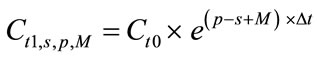
Capital growth model describes the concentration of capital at a point in time. In companies that continue their operations, capital grows according to the equation (1) ([15]: p. 133)1:
 , (1)
, (1)
where:
Ct0—the beginning concentration of capital [expressed in monetary terms] in the time moment t0Ct1,s,p,M—the ending concentration of capital [expressed in monetary terms] in the time moment t1, which has been subdued to natural dispersion “s” (risk), risk premium “p” and a management variable “M” through the time period ∆tS—dispersion variable (risk) [expressed as 1/year]P—risk premium, p = E(s) [expressed as 1/year]M—management variable [expressed as 1/year]∆t—time period between time moments: t0 and t1 [expressed in years].
According to M. Dobija [3] “the variables s and m represent active work of the natural forces (–s) and the active outer work that can restrain the dispersion (m) (…) the constant p symbolizes a potential. The potential p can yield fruit, provided the diffusion s is counterbalanced by the work m”. The author claims that the ex ante size of the potential p equals to 8%/yr. That potential represents the fair capital growth rate. Modified return on assets ratio may serve as proxy for risk premium estimation and as empirical research done at the 20 year period suggests, the yearly size of ex post p for average risk level conditions may be described as the 99.9% confidence interval: (8.08%/yr ; 8.74%/yr) [16].
Capital will grow and increase its concentration only if: “p – s + M > 0”. That condition represents at the same time ex post rate of return on invested capital, and also at the same time capital growth rate expressed in [1/year].
Recalling that capital is embodied in assets the equation (2) may be stated ([16]: p. 95):
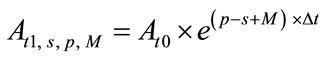 , (2)
, (2)
where:
At1,s,p M—the net cost of assets in the time moment t1 (these assets embody capital, that is subdued to natural dispersion “s” (risk), risk premium “p” and a management variable “M” through the time period of ∆t = t1 – t0, e.g. 1 year);
At0—the net cost of assets in the time moment t0.
Further, knowing that “er ≈ 1 + r”, the equation (2) may be rearranged into equation (3):
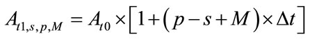 . (3)
. (3)
The reconciliation of units and their dimensions used in the equation (3) clearly shows that the value of assets, i.e. the concentration of capital in resources, is expressed in monetary units in the beginning and in the end of a period under consideration. That is proven by the equation (4):
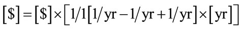 . (4)
. (4)
In the formula (3), factors “p” (risk premium), “s” and “M”, taken together, create an empirical growth rate, which is expressed in [1/year] terms. That growth rate is in fact the rate of return on capital in a one-year period or the rate of return on assets if the previously described understanding of capital is accepted. Thus, by skipping factors “p”, “s” and “M”, the equation (5) may be written:
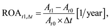 (5)
(5)
where:
At1—the net cost of assets in the time moment t1At0—the net cost of assets in the time moment t0∆t = t1 – t0ROAt1,∆t—the rate of return on capital embodied in assets calculated in t1 time moment realized in the time period ∆t.
The increase in concentration of capital embodied in assets “At1 – At0” equals to the realized income in a considered period “I∆t”. Since business processes are continuous processes rather than discrete, it seems more appropriate to compare the realized income “I∆t” to the average value of capital (equity or debt that is embodied in assets) in a considered period “Aav”. The change in the denominator results in the equation (6):
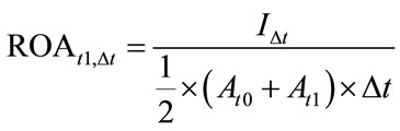 , (6)
, (6)
where:
I∆t—the realized income before extraordinary items in the period ∆tAt1, At0, ∆t and ROAt1,∆t as above.
The category of income to be used in the numerator of the formula number (6) should represent the normal operating conditions of each company. Therefore the impact of extraordinary items should be eliminated. As a result one can use Pretax Income category. Another advantage of that formula is that it is an income level before distribution of profit i.e. before dividends and taxes were paid. Summing up, Pretax Income category relates to the growth of capital in a particular period for normal risk level conditions.
3. Research Hypotheses
As M. Dobija suggests in his quoted publications, i.e. [2] and [3], as well as in numerous other, the potential for capital growth is a constant value of 8% per year. The research suggests that this potential is not realized as a rate of return on capital/assets for every company in each subsequent year [16,17]. Rather, the eight percent empirical growth rate is realized in large populations in average risk level conditions in long time periods. Companies in certain periods randomly realize higher or lower capital growth rate than the potential specified by M. Dobija in his model, however in the long term in large populations, average empirical capital growth rate will float towards the average. Therefore it may be stated that investors should not drain companies in more prosperous periods. They should rather allow firms to accumulate capital for times of crisis, as these periods will be followed by poorer ones.
The paper addresses a question, whether average ROA realized by companies in the years prior to the recent crisis were higher than the average rates in preceding five year periods. That might have led investors to seek for higher returns. The result was the recent textbook crisis as P. Viernimmen et al. claims.
The researched sample consists of companies constituting Standard & Poor’s SmallCap 600, Standard & Poor’s MidCap 400, Standard & Poor’s 500 indices on 31st January 2008. Audited, filed financial statements come from years 1999-20072. These financial statements were obtained from COMPUSTAT database (North America set, software: Research Insight version 8.3, 0.75).
Null hypotheses are presented in table 1, whereas alternative hypotheses are presented in table 2.
The average rates of return on assets in the researched time periods are presented in table 3.
In order to verify all of the presented hypotheses a test of the differences between two population means was applied—equation (7), with the usage of the modified degrees of freedom—equation (8) [18]:
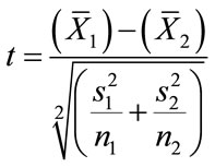 , (7)
, (7)
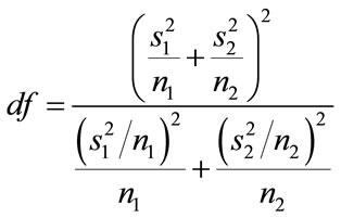 , (8)
, (8)
where:
t—value of the test statistics (t-Student distribution)df—modified degrees of freedoms—standard deviationn—number of observations,
 —arithmetic average from the sample. Subscripts 1 and 2 relate to compared populations.
Table 4 includes the overall number of observations in each index according to the period. Table 5 includes values of t-statistics rounded to the fourth digit after a comma and the number of modified degrees of freedom rounded to the nearest unit. For the one-sided test the critical t-value (t-Student distribution) for significance levels of: α = 0.100, α = 0.050, α = 0.025, α = 0.010, α = 0.005 and the number of degrees of freedom approaching ∞, equals to: ±1.282, ±1.645, ±1.960, ±2.326, ±2.576 respectively (plus sign if the order of averages in the numerator is as in null hypotheses). Table 6 presents the statistical decisions whether the researched data rejects the null hypothesis or whether the data fails to reject it at a given significance level.
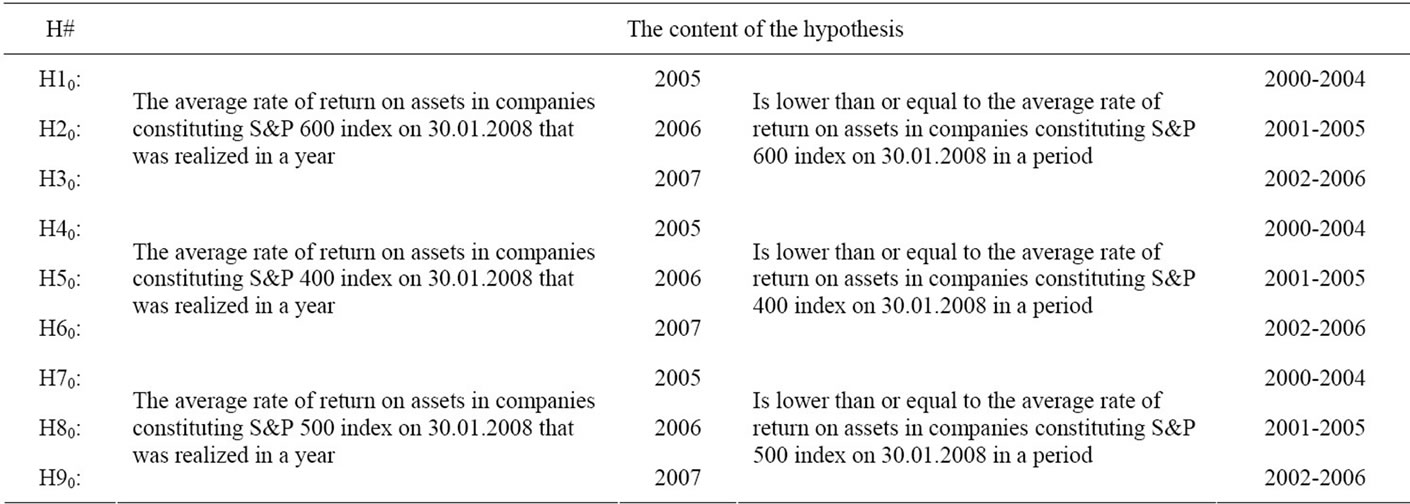
Table 1. Null hypotheses.

Table 2. Alternative hypotheses.
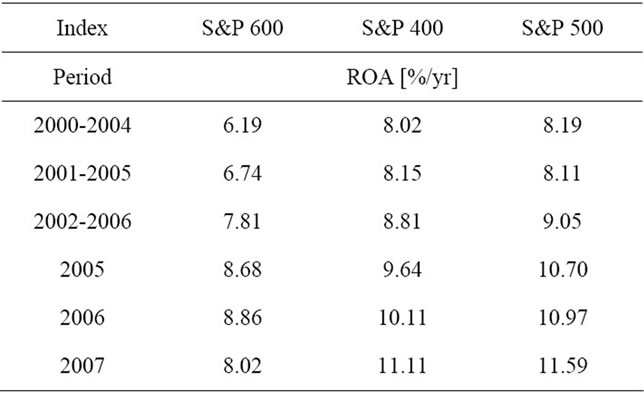
Table 3. Average rates of return on assets in each index according to the period.
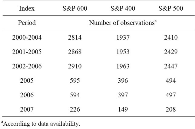
Table 4. The number of observations in each index according to the period.

Table 5. T-statistics and the numbers of modified degrees of freedom for each of the hypotheses.
The statistical hypotheses testing clearly showed that eight out of nine null hypotheses were rejected on the basis of researched data and only one null hypotheses was not rejected. The average rates of return on assets in companies constituting S&P 600 index on 30.01.2008 that were realized in a year 2005 and 2006 were statistically higher than in periods 2000-2004 and 2001-2005
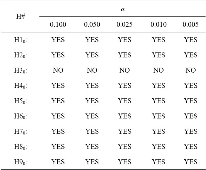
Table 6. Decision on the rejection of null hypotheses on the basis of researched data.
respectively. Similarly the average rates of return on assets in companies constituting S&P 400 index on 30.01. 2008 that were realized in a year 2005, 2006 and 2007 were statistically higher than in periods 2000-2004, 2001-2005 and 2002-2006 respectively. The same applies for companies constituting S&P 500 index on 30.01. 2008—the average rates of return on assets in companies constituting that index on 30.01.2008 that were realized in a year 2005, 2006 and 2007 were statistically higher than in periods 2000-2004, 2001-2005 and 2002-2006 respectively. Only the third hypothesis cannot be rejected on the basis of presented data—the average rate of return on assets in companies constituting S&P 600 index on 30.01.2008 that was realized in a year 2007 was lower than or equal to the average rate of return on assets that was realized in a period 2002-2006. The 2007 capital growth rate equaled to 8.02%/yr in that sample, whereas the one realized in the period 2002-2006 equaled to 7.81%/yr, which is still higher in nominal values.
It is worth to mention that year by year average capital growth rates increased for companies constituting S&P 400 and S&P 500 indices, starting from 9.64%/yr in 2005 though 10.11%/yr in 2006 ending with 11.11%/yr in 2007 in case of the former and starting from 10.70%/yr in 2005 though 10.97%/yr in 2006 ending with 11.59%/yr in 2007 in case of the latter. Average capital growth rate in companies constituting S& P600 index equaled to 8.68%/yr in 2005 and increased to 8.86%/yr in 2006, after which it dropped to 8.02%/yr in 2007.
4. Capital Growth Rate Estimation
The next step is to construct confidence intervals for capital growth rates for each of the index in each of the years under consideration. Average return on assets in a sample consisting of a particular index (S&P 600, S&P 400 and S&P 500) may serve as an estimator for capital growth rate in the population of small, medium and large well managed companies respectively. According to the central limit theorem the formula based on the standard normal distribution may be used to estimate population mean, when sampling from any distribution with unknown variance and when sample size is large. The numbers of observations in each index in each of years under consideration are presented in table 7. It may be claimed that the sample sizes are large.
The two-sided confidence interval for the population capital growth rate is constructed according to the formula number (9) (compare [19]):
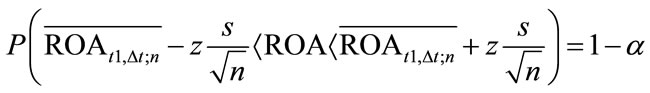 (9)
(9)
where:
z—value of the test statistics (normal distribution)s—standard deviationn—the number of observations,
 —average rate of return on capital embodied in assets calculated in t1 time moment (the end of the calendar year for which the average ROA is calculated) realized in the time period ∆t (the calendar year for which the average ROA is calculated) from n observations in a particular indexROA—capital growth rate in the population under consideration;
1 – α—confidence interval.
Average rates of return on assets for each year and each index are presented in table 8, whereas standard deviations are presented in table 9.
Confidence intervals for capital growth rates in each index in each of the years for the degree of confidence equal to 0.99 are presented in table 10 (1-year periods), in table 11 (5-year periods) and in table 12 (8-year periods). Relative precisions of estimations are included in tables 13-15 respectively.
Relative precisions of estimations in case of 1-year periods it is higher than 10% and as a result estimation is completely wrong. That proves the need for long time horizons research. In case of 5-year periods relative precisions of estimations only in two situations are above 10%. In all other situations these are below 10% but still above 5%, which is not satisfactory, as it cannot be claimed that estimation is safe and fully acceptable.
Even in the case of 8-year periods relative precisions of estimations are above 5% in case of the degree of confidence equal to 99%.
By limiting the degree of confidence to 90%, one can achieve relative precision of estimations below 5% for
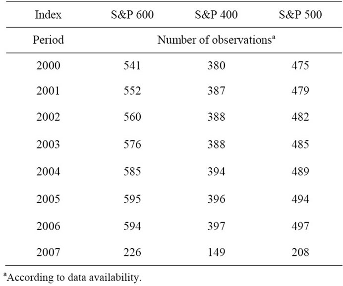
Table 7. The number of observations in each index in each year.
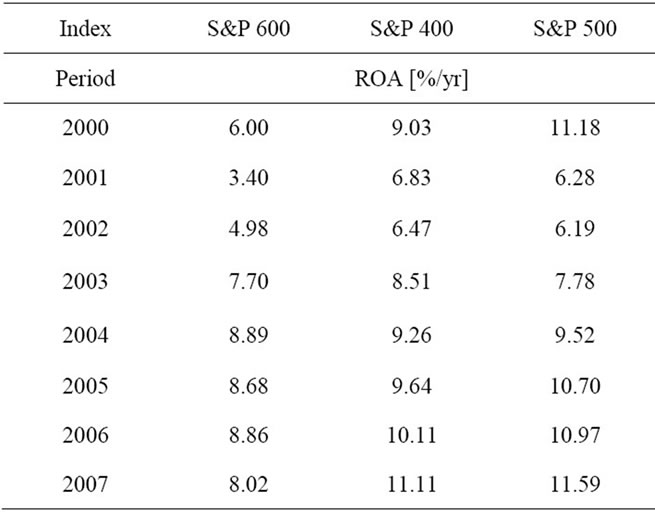
Table 8. Average rates of return on assets in each index according to the year.
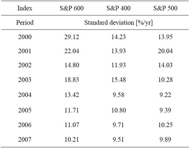
Table 9. Standard deviations of the average rates of return on assets in each index according to the year.
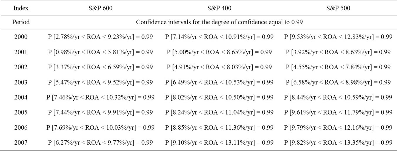
Table 10. Confidence intervals for capital growth rate (1-year periods).
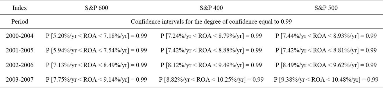
Table 11. Confidence intervals for capital growth rate (5-year periods).
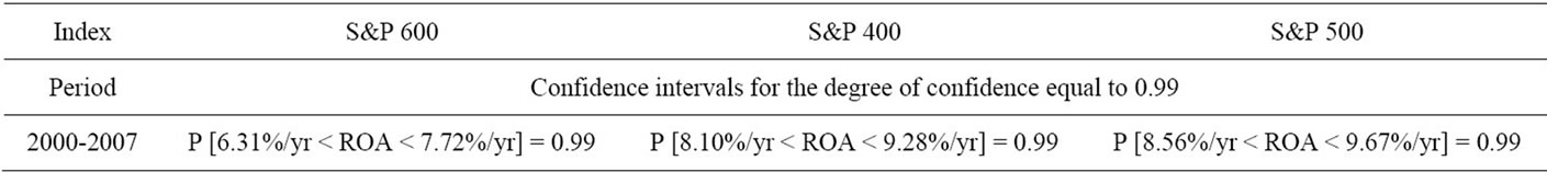
Table 12. Confidence intervals for capital growth rate (8-year periods).
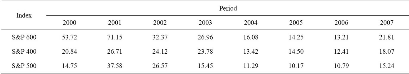
Table 13. Relative precision of estimation in % (1-year periods, degree of confidence equals to 0.99).
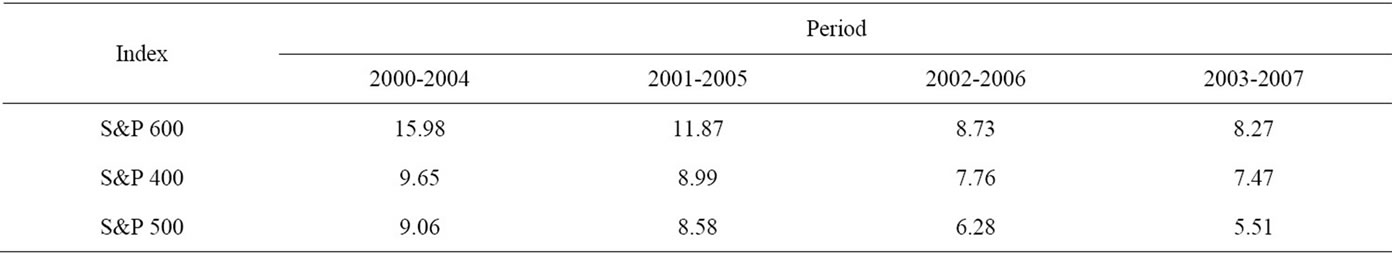
Table 14. Relative precision of estimation in % (5-year periods, degree of confidence equals to 0.99).
indices S&P 400 and S&P 500, which is a level of safe and fully acceptable estimation (tables 16 and 17). Another possibility is to increase the size of the sample, which was done in [16,17,20].
5. Conclusions
Capital in economy—according to the contemporary approach—is understood as an abstract homogeneous ability to perform labor. Capital is embodied in assets, which are concrete and heterogeneous. The concentration of capital comprises the value of assets. Capital is subdued to a number of laws, such as: the conservation principle the dispersion principle and the capital growth principle. The conversion principle states that the total amount of capital remains constant in an isolated system. The increase of initial capital in an enterprise may only be caused by the exchange at the free, efficient market. The dispersion principle states that the initial value of capital spontaneously and randomly declines.
Capital growth principle stems from the assumption that economy is a non-zero game. According to M. Dobija the fair capital growth rate in an average risk level conditions equals to the potential of 8%. The potential is one of the three factors that condition the concentration of capital in a particular time moment. The remaining
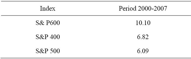
Table 15. Relative precision of estimation in % (8-year periods, degree of confidence equals to 0.99).
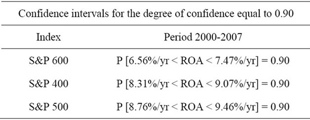
Table 16. Confidence intervals for capital growth rate (8- year periods).
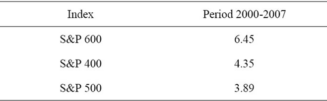
Table 17. Relative precision of estimation in % (8-year periods, degree of confidence equals to 0.90).
two factors are natural dispersion and management variable. These three factors determine the rate of return on invested capital, which is a random number for a particular company.
The potential may be empirically estimated. Capital average growth rates of companies operating in average level conditions fluctuate around the potential, assuming that large populations over long time periods are tested. Individual capital growth rates are random numbers, i.e. cannot be forecasted with certainty. The estimation of the potential is in fact the estimation of the fair average capital growth rate in large populations. The theory of capital states that the higher capital growth rates in some periods will be followed by the lower growth rates in other periods.
Therefore higher capital growth rates in some periods cannot be used to justify the drain of profits from companies, as in other periods returns will reverse and move towards long term average. P. Viernimmen et al. claimed that the 2007 crisis was a textbook case, where greedy investors sought increasingly higher returns and were never satisfied when they had enough. Empirical research suggests that capital growth rates in years prior to crisis were higher than the average capital growth rates in the preceding years. The nine hypotheses were tested in order to prove the assumption. In case of Standard & Poor’s MidCap 400 index and Standard & Poor’s 500 index the capital growth rates that were realized in years prior to crisis, i.e. in years: 2007, 2006, 2005 were statistically higher than the average growth rates in preceding 5-year periods, i.e. in periods: 2002-2006, 2001-2005 and 2000-2004 respectively. In case of Standard & Poor’s SmallCap 600 index the capital growth rates that were realized in years prior to crisis, i.e. in years: 2006, 2005 were statistically higher than the average growth rates in preceding 5-year periods, i.e. in periods: 2001-2005 and 2000-2004 respectively. Only in case of Standard & Poor’s SmallCap 600 index the realized capital growth rate in year 2007 was not statistically higher than the average growth rates in a period 2002-2006.
Additionally 40 confidence intervals for capital growth rates were constructed. These clearly show that capital growth rates are concentrated around the potential, as it is proved in [16,17,20], where longer time horizons are investigated. Confidence intervals for capital growth rates equal to (6.56%/yr; 7.47%/yr), (8.31%/yr; 9.07%/ yr), (8.76%/yr ; 9.46%/yr) in case of S&P 600, S&P 400 and S&P 500 indices respectively (the degree of confidence 0.90, 8-year periods analyzed). It is clearly visible that larger companies offer relatively greater potential for growth than the middle ones and middle ones offer higher potential for growth than smaller ones. That is in line with assumptions described in introduction that S&P 500 index includes 500 leading companies in leading industries of the US economy. On the other hand S&P 600 index covers small cap segment of the market, which is characterized by poor trading liquidity and financial instability. S&P 400 index is in between the two indices.
It is particularly important to learn that capital growth rates fluctuate around the potential of growth. That knowledge may protect individual investors—citizens—from losses. Greedy institutional investors frequently tempt citizens with constant higher than average returns. The past pattern of returns may not continue in future periods. The constant increase in capital growth rates may even act as a warning sign. The theory of capital explains the phenomenon—capital growth rates fluctuate around the potential of growth.
REFERENCES
- P. Viernimmen, P. Quiry, M. Dallocchio, Y. Le Fur and A. Salvi, “Corporate Finance: Theory and Practice,” John Wiley & Sons Ltd., Chichester, 2009.
- M. Dobija, “Abstract Nature of Money and the Modern Equation of Exchange,” Modern Economy, Vol. 2, No. 2, 2011, pp. 142-152. doi:10.4236/me.2011.22019
- M. Dobija, “Labour Productivity vs Minimum Wage Level,” Modern Economy, Vol. 2, No. 5, 2011, pp. 780-787. doi:10.4236/me.2011.25086
- “S&P Indices: The S&P MidCap 600,” Access on 2 January 2012. http://www.standardandpoors.com/indices/sp-smallcap-600/en/eu/?indexId=spusa-600-usduf--p-us-s--
- “S&P Indices: The S&P MidCap 400,” Access on 2 January 2012. http://www.standardandpoors.com/indices/sp-midcap-400/en/eu/?indexId=spusa-400-usduf--p-us-m--
- “S&P Indices: The S&P MidCap 500,” Access on 2 January 2012. http://www.standardandpoors.com/indices/sp-500/en/eu/?indexId=spusa-500-usduf--p-us-l--
- I. Fisher, “The Nature of Capital and Income,” Augustus M. Kelly Publisher, New York, 1965, pp. 53-57.
- E. von Böhm-Bawerk, “Capital and Interest, Vol. 2: Positive Theory of Capital,” Libertarian Press, South Holland, 1959, pp. 16-66.
- E. Majewski, “Capital: The Set of Core Phenomena and Concepts in Economy,” 4th Edition, E. Wende i ska, Warszawa, 1914.
- S. T. Skrzypek, “The Concept of Capital in Literature,” Nakł. Towarzystwa Naukowego, Pomerania, 1939.
- C. Bliss, “Capital Theory and the Distribution of Income,” North-Holland Publishing Company, Oxford 1975.
- Y. Ijiri, “Segment Statements and Informativeness Measures: Managing Capital vs Managing Resources,” Accounting Horizons, Vol. 9, No. 3, 1995, pp. 55-67.
- M. Dobija, “Abstract Nature of Capital and Money” In: L. M. Cornwall, Ed., New Developments in Banking and Finance, Nova Science Publishers, Inc., New York, 2007, pp. 89-114.
- F. L. Lambert, “Shuffled Cards, Messy Desks, and Disorderly Dorm Rooms—Examples of Entropy Increase? Nonsense!” The Journal of Chemical Education, Vol. 76, No. 10, 1999, pp. 1385-1387. doi:10.1021/ed076p1385
- M. Dobija, “Fair Value as a Criterion of Truth in Economic Theory” In: W. Adamczyk, Ed., Dążenie do Prawdy w Naukach Ekonomicznych, Akademia Ekonomiczna w Krakowie, Kraków, 2006, pp. 125-150.
- B. Kurek, “An Adjusted ROA as a Proxy for Risk Premium Estimation—The Case of Standard and Poor’s 1500 Composite Index,” Cracow University of Economics, Krakow, 2010, pp. 87-103.
- B. Kurek, “The Risk Premium Estimation on the Basis of Adjusted ROA,” In: I. Górowski, Ed., General Accounting Theory: Evolution and Design for Efficiency, Academic and Professional Press, Warsaw, 2008, pp. 375-392.
- R. A. DeFusco, D. W. McLeavey, J. E. Pinto and D. E. Runkle, “Hypothesis Testing,” In: Ethical and Professional Standards and Quantitative Methods (CFA Program Curriculum), Pearson Publishing, Boston, 2007.
- Z. Hellwig, “Elements of Probability Calculus and Mathematical Statistics,” 8th Edition, PWN, Warszawa, 1978, p. 214.
- B. Kurek, “Hypothesis of Deterministic Risk Premium,” Ph.D. Thesis, Cracow University of Economics, Kraków, 2011.
NOTES
1Compare also [2] and [3].
2Financial statements are from the period 1999-2007, whereas periods in statistical tests start in year 2000. That stems from the calculation of the arithmetic average of assets as described in Equation (6).