Modern Economy
Vol. 3 No. 3 (2012) , Article ID: 19155 , 12 pages DOI:10.4236/me.2012.33036
The Optimal Timing of the Transition to New Environmental Technology for Economic Growth
1College of Arts and Sciences, The University of Tokyo, Tokyo, Japan
2Graduate School of Economics, Kyoto University, Kyoto, Japan
Email: maeda@global.c.u-tokyo.ac.jp, makiko.nagaya@gmail.com
Received February 26, 2012; revised March 13, 2012; accepted March 29, 2012
Keywords: Environmental Quality; Optimal Stopping; Technological Change
ABSTRACT
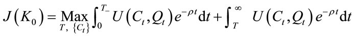
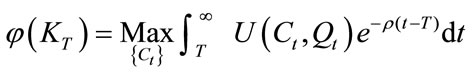
This study investigates the best timing for technological change affecting environmental quality in economic development. We develop a model that addresses the transition of environmental technology from an old system to a new one. Findings obtained are innovative in that they depict when as well as how transition to new environmental technology occurs. It demonstrates that the timing is endogenous and characterized by the properties of the economy: in particular, the optimal technology transition timing depends upon whether the economy is developing or developed.
1. Introduction
Since the 1970s, many researchers have worked on resource and environmental issues relating to economic growth. Classical studies that incorporated exhaustible resources into the Ramsey model include Dasgpta and Heal [1], Stiglitz [2], Solow [3], and others. These studies pioneered theoretical investigation of the economic growth possible with natural resource constraints.
In the 1980s, the environment began to be recognized as an important factor that determines the trajectories of growth. At the same time, the theory of economic growth began to change: “endogenous change” became a central issue in economic literature: Romer [4], Lucas [5], and others, established the “endogenous economic growth theory.” These two streams converged in a series of studies after the late 1990s, addressing the central role that endogenous technological change plays in sustainable development.
Barbier [6], and Tahvonen and Salo [7] developed their endogenous growth models combined with resource constraints, highlighting the critical role of technology policy. On the other hand, Bovenberg and Smulders [8], Schou [9], Groth and Shou [10], and Grimaud and Rougé [11] introduced “knowledge” or “know-how” into their models of production sectors, and discussed how this knowledge accumulation would contribute to mitigating environmental constraints1.
Cunha-e-Sá and Reis [15] contributed to the literature in their investigation of the optimal timing of adoption of new environmental technologies: as the economy grows, new pollution-abating technology becomes indispensable; it requires investment efforts at the time of deployment; the optimal timing will be determined endogenously. In fact, they incorporated “environmental quality” and “clean technology” into a typical Ramsey-type model. They assumed that the level of clean technology could change discontinuously once the “upgrade” occurred. Upgrading the technology might require costs such as depreciation of capital, investment for research and development, and the like. Thus, consideration of the net benefit of the technology determines the optimal timing of the upgrade.
While Cunha-e-Sá and Reis underlined the signifycance of “the optimal timing” in the framework of the environment and economic growth, some debatable issues remain. The most debatable issue is that technological change in clean technology is represented by an abrupt increase in the level of clean technology. Allowing such a sudden change of the technology level implies that the change does not require accumulation of some stocks; that is, the change is not due to stocks, but is due to the temporal flow. More specifically, the nature of technological change in clean technology in Cunha-e-Sá and Reis has nothing to do with any stocks of capital, knowledge, know-how, human capital, etc., and thus cannot be endogenously described. This nature contrasts with the fundamental idea of modern endogenous growth theory: in this theory, one of the key drivers for economic growth is intellectual capital. In this respect, their treatment of technological change for clean technology seems oldfashioned. Another important issue is their treatment of investment cost. In their model, the required cost of technological change is represented as a fixed cost, the amount of which is proportional to the difference between old and new clean technology levels. In addition, it is taken into account as a part of the objective function. This setting seems strange: as long as we assume a closed economy, the investment cost must be paid by somebody in the economy, meaning that the objective function should not explicitly include the cost; the investment cost should be treated as a decline in consumption or in asset holdings. Cunha-e-Sá and Reis do not seem to provide any explanation of this point. For the outline of their model, see Appendix 6.
Including investment cost in the objective function causes another problem. In the Ramsey model, the objective function is basically the sum of temporal utilities that are discounted to the present. It does not have any unit. If we want to subtract investment costs from it, the unit of the cost—usually in monetary terms—must be transformed somehow. The coefficient for the transformation should be interpreted as a shadow price of the clean technology investment. Thus, it must naturally have a dynamic and be determined endogenously. However, in Cunha-e-Sá and Reis it is treated as a fixed parameter, but they do not provide a clear explanation of this point.
An analysis of the studies of Cunha-e-Sá and Reis provide a promising direction for further research: their model may be modified by focusing on the acceleration (changes in the growth rate) of clean technology, rather than the change in the technology level itself, and also by working on a traditional objective function that simply consists of the sum of discounted temporal utilities. It is our purpose that we explore such a direction.
This study highlights the choice of timing for technological change affecting environmental quality in economic development. Based on the intent and mathematical treatment of Cunha-e-Sá and Reis, we develop an analytical model that addresses the optimal timing of the transition of environmental technology from old to new.
The paper is organized as follows: Section 2 describes the model. Section 3 investigates the dynamics of the model through dynamic programming and maximum principle techniques. Section 4 puts forth three propositions and discusses their implications. Section 5 summarizes and concludes with the study’s findings.
2. The Model
The study uses a Ramsey-type model. The economy is closed, with no international trade. The population is assumed to be constant. Let us define notations as follows:
Y: Production output K: Capital C: Consumption Q: Environmental quality a: Environmental technology level
2.1. Representative Agent
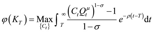
A representative economic agent represents the household whose time-additive utility is determined by not only consumption (C) but also “environmental quality” (Q). More specifically, we define2:
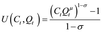 ,
,  (1)
(1)
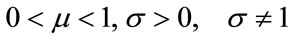
where σ represents the magnitude of the elasticity of marginal utility with respect to .
.
Note that subscript t indicates time in years. This applies throughout.
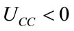
We impose the following restrictions for the utility function to be increasing and strictly concave in Ct and Qt3.
 .
.
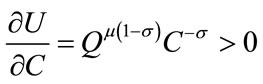
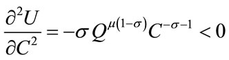
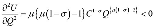
These restrictions determine signs of partial derivatives of the utility function as follows:
 ,
,  ,
, and
and .
.
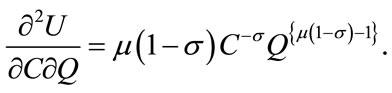
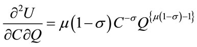
The cross derivative is:
 the sign of which remains undetermined. In fact, the sign depends on the magnitude of the elasticity of marginal utility (σ). We will discuss this point later.
2.2. Production Sector
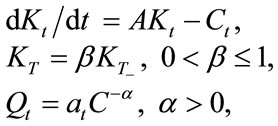
The production sector is described rather in a simple manner: we assume that output is proportional to capital input; that is:
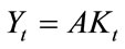 . (2)
. (2)
With this production function, capital accumulation is subject to the following:
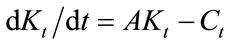 . (3)
. (3)
2.3. Environmental Quality and Clean Technology
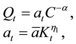
We now introduce the roles of environmental quality and technology. We assume that the environmental quality (Q) is a function of consumption (C) as well as the “environmental technology level” (a). The relationship is assumed as follows:
 ,
, . (4)
. (4)
This functional form indicates that environmental quality declines as consumption grows, but that it may improve as environmental technology progresses.
The progress of the environmental technology level itself may occur as the economy grows. Considering capital stock (K) as a proxy of economic growth, we assume that the growth rates of a and K are proportional to each other:
 .
.
Introducing a positive coefficient η, the relation is written as follows:
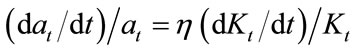 .
.
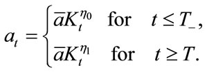
Notice that the coefficient determines the rate of environmental technology progress together with that of capital accumulation. Thus, if the economy has an internal mechanism that changes the coefficient, the mechanism accelerates the technological progress. The change in the coefficient is not necessarily gradual. Rather, it may be discontinuous, and may happen in an innovative manner. We call this type of discontinuous change in the rate of environmental technology progress “transition.” Since it is a result of some innovation, we may assume that it may happen at one time in the infinite time horizon with a huge capital expenditure. The expenditure includes not only investing money in the usual way, but also scrapping existing physical capital because part of the physical capital may become obsolete and old-fashioned once such an innovation occurs.
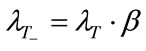
Let T denote the time of transition. For the purpose of mathematical treatment, let us introduce a notation  such that:
![]() .
.
Transition of environmental technology is represented by an abrupt change of the coefficient that links two growth rates of technology and capital stock to each other. More specifically, the following relation holds true:
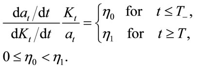 (5)
(5)
The relation indicates that the environmental technology level (a) is written as a function of capital stock (K) as follows:
 (6)
(6)
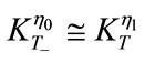
Let  denote the capital stock at the time of
 , that is:
![]() .
.
As discussed above, the transition is a result of onetime expenditure decision that includes scrapping of existing physical capital. The expenditure is thus described as substantial decline in the present capital. More specifically, we assume that following relationship holds true:
 . (7)
. (7)
The coefficient β represents the rate of depreciation of existing physical capital at the time of transition.
Note that in Equation (6), ![]() represents an absolute level of the technology. While we need to assume a constant value somehow for it as a modeling frame, the absolute level itself does not play any important role in the model. Only changes in the level play a role. Thus, the value of
represents an absolute level of the technology. While we need to assume a constant value somehow for it as a modeling frame, the absolute level itself does not play any important role in the model. Only changes in the level play a role. Thus, the value of  itself is not important and may remain undetermined. Instead, we introduce the following restriction:
 . (8)
. (8)
This restriction indicates continuity of the technology level at the very moment of transition T. We assume that ![]() is fixed ex post facto so that Equation (8) holds true.
is fixed ex post facto so that Equation (8) holds true.
2.4. Optimization
Given the above setting, the representative economic agent chooses the consumption path as well as the time of transition. While the decision for the consumption path is a typical optimal control, the decision for the choice of the time of transition constitutes an optimal stopping problem. The economy follows the optimal solution of the following dynamic programming problem.
 (9)
(9)
s.t. ,
, 
The problem has control variables ![]() and T and a state variable
and T and a state variable![]() . Therefore, we can solve the problem by the following procedure:
. Therefore, we can solve the problem by the following procedure:
First step: optimize the value function for a given capital stock for after-transition.
 (10)
(10)
Second step: optimize the value function for a given transition time for the whole time horizon.
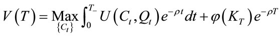 (11)
(11)
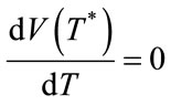
Final step: maximize (11) with respect to T.
![]() (12)
(12)
The next section investigates the details of the procedure.
3. Analysis
Suppose that technology transition has already occurred at time T. Capital stock at the time is fixed at the level of KT. The optimization problem thereafter is described as follows:
 (13)
(13)
s.t. 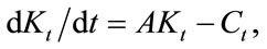
 is given; t ³ T.
To solve the problem, let us introduce the currentvalued Hamiltonian as follows:
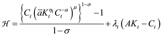 . (14)
Note that λt represents a current-valued shadow price of capital.
First order necessary conditions for the optimality are written as follows:
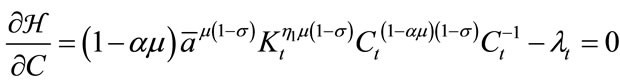 , (15)
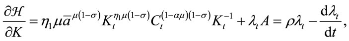 (16)
(16)
 . (17)
Combining Equations (15) and (16), we have the following differential equation with respect to :
:
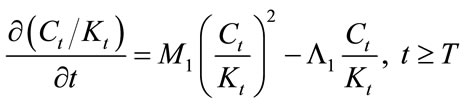 , (18)
where
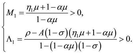
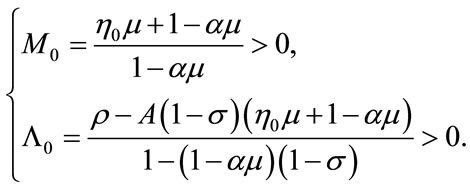
Solving Equation (18) with the condition (17), the solution is obtained as follows:
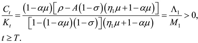 (19)
(19)
The above solution shows that the proportion of consumption to capital stock remains constant after the technology transition. This rule suggests that consumption and capital stock grow at the same rate after the transition. In fact, their growth rates are found as follows:
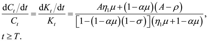 (20)
(20)
Employing Equations (19) and (20), the integral of (13) is obtained as follows:
 (21)
(21)
Having obtained  as Equation (21), we are ready to work on (11). Let us rewrite the problem:
 (22)
(22)

T is given; .
.
Again, we introduce the current-valued Hamiltonian, and derive first order necessary conditions as follows:
 , (23)
 , (24)
 . (25)
Because capital stock changes discontinuously at time T, so does its shadow price. It is easily shown that:
 . (26)
Notice that Equations (23) and (24) are similar to Equations (15) and (16), respectively. The only difference is that we replaced  with
with . Thus, they provide a similar differential equation to (18):
 (27)
(27)
where
Due to Equations (7), (8), and (26), the values of  and
and  must satisfy the following:
 . (28)
Solving Equation (27) with its terminal condition (28), we obtain the following:
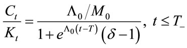 (29)
(29)
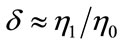
where
 (30)
(30)
From Equation (29), we obtain the dynamics that capital stock must follow before the transition happens, as follows:
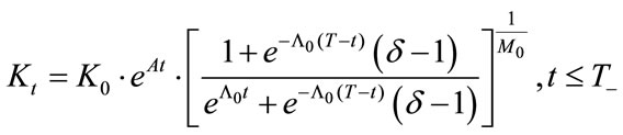 . (31)
This enables us to evaluate V(T) in (22), which is a task in the next section.
4. Propositions
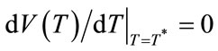
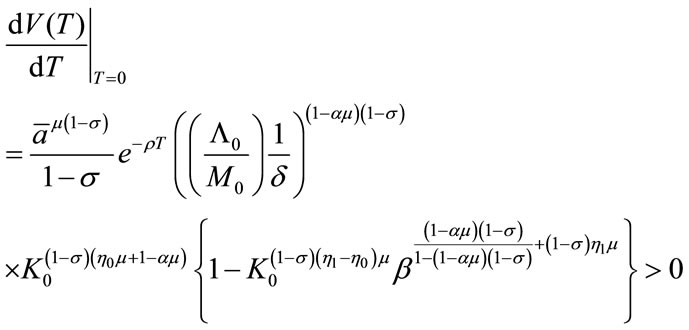
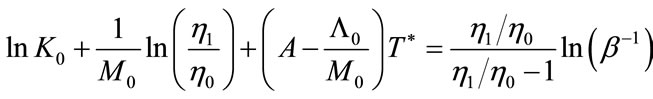
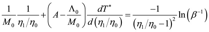
Our final step is to maximize V(T) of (22) with respect to T, given Equations (7), (21) and (31). The solution would provide the optimal time of transition T*. Although solving it analytically is not an easy task, examining the properties of the solution is rather easy. This is done by taking the derivative of V(T) with respect to T. From (22), we obtain the following:
(For the detail, see Appendix 2).
 (32)
(32)
To have a finite T*, we must have the following conditions:
 if
if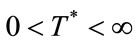 ,
,
 if
if .
.
These conditions lead to the following proposition.
Proposition 1
For a finite T* to exist, that is,  , the following condition is necessary:
 . (33)
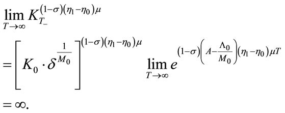
Conversely, if 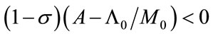 holds true, then the transition to new environmental technology never occurs (i.e. T* = ∞).
(For proof, see Appendix 3).
Let us examine the implication of the proposition. The necessary condition (33) is equivalent to the following:
Either  and
and 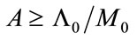
or  and
and 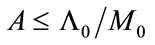 hold true.
From Equation (29), we have:
 which implies:
 (29’)
(29’)
Thus, we have:
 if and only if
 .
.
Notice that  represents the average consumption propensity just before the transition. Then, we can further translate the condition (33) into the following conditions:
• If  holds true, the average consumption propensity just before the transition is less than or equal to
 .
.
• If  holds true, the average consumption propensity just before the transition is larger than or equal to
 .
.
As was shown in Section 2, s represents the magnitude of the elasticity of marginal utility and determines the sign of the cross derivative of the utility function as follows:
When  holds true, the marginal utility with respect to environmental quality (ðU/ðQ) turns out to be increasing in consumption. (That is, ð(ðU/ðQ)/ðC > 0.) This means that the potential of utility improvement with respect to environmental quality improvement is higher when the level of consumption is high, than otherwise. This also implies that a higher consumption would yield a higher marginal value of environmental quality. A similar interpretation can result by transposing C and Q: the marginal utility with respect to consumption (ðU/ðC) is increasing in environmental quality, meaning that the potential of utility improvement with respect to the increase in consumption becomes higher when the level of environmental quality is high. In short, marginal value of environmental quality (consumption) becomes higher as consumption (environmental quality, rep.) grows. In this sense, consumption and environmental quality are complementary in the course of economic development. A society prefers more environmental quality improvement as its consumption grows.
On the other hand, when  holds true, the marginal utility with respect to environmental quality (ðU/ðQ) is decreasing in consumption. (That is, ð(ðU/ðQ)/ðC < 0.) This means that a higher consumption would yield a lower marginal value of environmental quality. Again, transposing C and Q, we can say that a higher environmental quality would yield a lower marginal value of consumption. In short, marginal value of environmental quality (consumption) becomes lower as consumption (environmental quality, rep.) grows. This situation indicates that consumption and environmental quality are inversely proportional values to each other. A society considers environmental quality to be less important as its consumption grows.
Intuitively speaking, a society with the condition of  is said to care about the environment in conjunction with consumption growth while one with the condition of
  is not.
Combining these interpretations for  and s together, Proposition 1 is interpreted in words as follows:
Interpretation of Proposition 1
For the transition to occur within a finite time horizon, the economy must be in either of the following two situations:
• The economy highly prefers environmental quality in conjunction with consumption growth, and its current average consumption propensity is lower than a certain value ( ).
).
• The economy prefers consumption to environmental quality, and its current average consumption propensity is higher than a certain value ( ).
).
Interpreting Proposition 1 in this way, we may surmise how the transition occurs. For the former case above, a lower consumption propensity indicates a higher saving rate. This implies that the economy wants to make the investment to develop capital stock. That is to say, the economy is in the phase of capital accumulation. Conversely, in the latter case above, the economy is depreciating its capital stock due to its higher average consumption propensity. In short, while technological transition may occur in the course of capital accumulation in the former case, it may also occur with capital depreciation in the latter case.
This conjecture is in fact justified by the following proposition.
Proposition 2
Suppose that  holds true. If the following conditions hold true:
Either  and
and
 , (34)
or  and
and
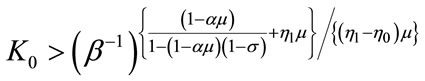 , (35)
then there exists an optimal transition time T* such that 0 < T* < ∞, which is obtained by solving the following equation:
 (36)
(36)
Moreover, the capital stock at the time is provided as follows:
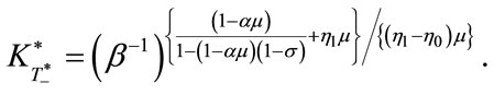 (37)
(37)
(For proof, see Appendix 4.)
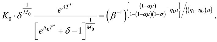
Knowing Equation (37), we can rewrite conditions (34) and (35) as follows:
if ,
,  must hold true, and (38)
if ,
,  must hold true. (39)
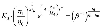
Similarly, Equation (36) is equivalent to the following:
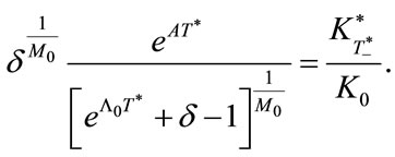 (40)
(40)
This equation indicates that for sufficiently large T*the following approximation holds true.

In addition, if  holds true4, then a further approximation is obtained:
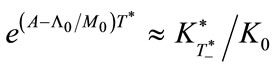 .
.
This approximation shows that:
for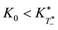 ,
,  , i.e.,
  , and for
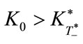 ,
,  , i.e.,
 .
.
However, we have already assumed that

is a sufficient condition for the existence of a finite T*. Thus, we find the above conditions are equivalent to conditions (38) and (39). Finally, we realize that Equation (40) is approximately consistent to conditions (38) and (39).
Another interesting finding is the independence of  from the initial capital stock
 . In fact, Equation (37) indicates that
  is a constant value and does not depend upon
 . This means that no matter from what level the economy starts growing (or shrinking), the transition of environmental technology occurs at the same capital stock level. That is to say, whether the economy is developed or developing, the transition occurs in the same economic conditions.
Our next attention, then, naturally proceeds to how the economy reaches the fixed capital stock level. We can find the answer from conditions (38) and (39): from these conditions, we can consider two types of dynamic behavior.
• In the case of , capital stock Kt increases and reaches the fixed level
  from below.
• In the case of , capital stock Kt declines and reaches the fixed level
  from above.
These are depicted as Figures 1 and 2. When  holds true (Figure 1), the capital accumulation is rather typical: it gradually increases with time. On the other hand, when
  holds true (Figure 2), the capital stock declines, which does not seem like typical growth. For the economy to be able to take such a path, it must have already developed sufficiently. In fact, the economy possesses huge capital, and is only consuming the capital.

Figure 1. Capital path for the case of 1 > σ.
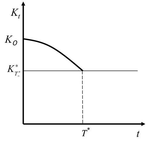
Figure 2. Capital path for the case of 1 < σ.
Such an economy must have once developed a large empire on the earth. Historical examples include the Holy Roman Empire and the British Empire.
We have already discussed the meaning of s above: whether s is less or greater than the unity divides the economy which cares about the environment in conjunction with consumption growth from the one which prefers consumption to environmental quality. In the former economy, as consumption grows, more environmental quality is needed. This motivates innovation in technology that improves environmental quality. On the other hand, in the latter economy, declining consumption motivates innovation. The reason for consumption declining is that the economy has been consuming its own assets. To recover the decline in utility, environmental quality improvement becomes necessary.
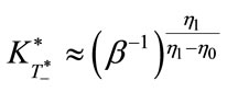
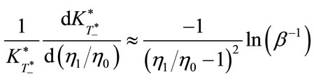
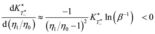
Finally, let us examine the sensitivities of the solution with respect to parameters that determine the evolution of environmental technology. The following proposition is obtained:
Proposition 3
Suppose that  holds true, and thus that there exists the optimal T* such that 0 < T* < ∞. Furthermore, suppose that the following approximations hold true:
 and
and .
.
Then, the derivatives of  and T* with respect to
  have signs as follows:
 , and (41)
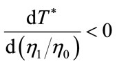 for
for ;
; for
for . (42)
(For proof, see Appendix 5.)
As defined in Equation (5),  and
and  are new and old coefficients, respectively, that link the growth rate of capital to that of the environmental technology level. The proportion
  represents the degree of the innovation. Intuitively, it tells how beneficial the transition to the new environmental technology is to the economy. Thus, it is easy to predict that a larger value of the proportion would make the optimal capital stock level for the transition smaller. Equation (41) clarifies this point.
The indications of (42) are consistent to (41). When , capital stock starts growing from a lower level and approaches the level of
 , which was shown by (38) and in Figure 1. Thus, a smaller
  would make the time of the attainment earlier. In contrary, when
 , initial capital stock is sufficient to the economy, as shown by (39), and no accumulation is needed. Declining capital stock eventually approaches the level of
  as was shown in Figure 2. Thus, a smaller
  would delay the time of the attainment.
These observations are depicted in Figures 3 and 4.
5. Conclusions
This study investigated the optimal timing of the transition in environmental technology from old to new, along with economic growth. The economy enjoyed consumption as well as environmental quality; thus, transition to an innovative environmental technology may benefit the economy, while the transition may impose a huge cost to the economy. Consideration of net benefit yields the optimal timing. The same idea has been proposed by Cunha-e-Sá and Reis (2007). We developed a model different from theirs in that:
• we focused on the acceleration (changes in the growth rate) of environmental technology, which is triggered by capital stock; and
• our treatment of the cost for the transition is rather simple, and thus helps reduce ad hoc parameters representing costs in the model.
We obtained three propositions depicting when as well as how the transition of environmental technology occurs. The timing is endogenous and is characterized by the properties of the economies, in particular whether the
Figure 3. The impact of the change in η1/η0 for the case of 1 > σ.
Figure 4. The impact of the change in η1/η0 for the case of 1 < σ.
economy is developing or developed. Findings are summarized as follows:
1) The primary determinant of whether the transition to new technology is needed or not is the degree of complementarity between environmental quality and consumption. A secondary determinant is the average consumption propensity. The necessity of the transition implies either a high degree of complementarity with a low consumption propensity or negative complementarity (i.e., inverse proportionality) with a high consumption propensity (Proposition 1).
2) Given the necessity of the transition to new technology, it may occur in two possible ways. One is that an environmentally developing economy would accumulate social capital and invest it in the development of the new technology. The other way is that a matured economy with sufficient capital and a high consumption rate would realize the need for environmental quality improvement eventually (Proposition 2).
3) The relationship between the optimal timing of the transition and the degree of the technology innovation depends upon the differences between the above two cases. For the former case, a higher degree of innovation leads to an earlier transition. However, for the latter case, the relationship is the opposite: a higher degree of innovation leads to a delay of the transition (Proposition 3).
These propositions depict how the acceleration (changes in the growth rate) of clean technology, rather than the change in the technology level itself, occurs. We believe this concept is innovative and thus addresses a possible direction of future research.
REFERENCES
- P. Dasgpta and G. M. Heal, “The Optimal Depletion of Exhaustible Resources,” Review of Economic Studies, Vol. 42, No. 5, 1974, pp. 3-28. doi:10.2307/2296369
- J. E. Stiglitz, “Growth and Exhaustible Resources: Efficient and Optimal Paths,” Review of Economic Studies, Vol. 41, No. 5, 1974, pp. 123-137. doi:10.2307/2296377
- R. M. Solow, “Intergeneration Equity and Exhaustible Resources,” Review of Economic Studies, Vol. 41, 1974, pp. 29-45. doi:10.2307/2296370
- P. M. Romer, “Endogenous Technological Change,” Journal of Political Economy, Vol. 98, No. 5, 1990, pp. S71- S102. doi:10.1086/261725
- R. E. Lucas Jr., “On the Mechanics of Economic Development,” Journal of Monetary Economics, Vol. 22, No. 1, 1988, pp. 3-42. doi:10.1016/0304-3932(88)90168-7
- E. B. Barbier, “Endogenous Growth and Natural Resource Scarcity,” Environmental and Resource Economics, Vol. 14, No. 1, 1999, pp. 51-74. doi:10.1023/A:1008389422019
- O. Tahvonen and S. Salo, “Economic Growth and Transitions between Renewable and Nonrenewable Energy Resources,” European Economic Review, Vol. 45, No. 8, 2001, pp. 1379-1398. doi:10.1016/S0014-2921(00)00062-3
- A. L. Bovenberg and S. Smulders, “Environmental Quality and Pollution-Augmenting Technological Change in Two-Sector Endogenous Growth Model,” Journal of Public Economics, Vol. 57, No. 3, 1995, pp. 369-391. doi:10.1016/0047-2727(95)80002-Q
- P. Schou, “Polluting Non-Renewable Resources and Growth,” Environmental and Resource Economics, Vol. 16, No. 2, 2000, pp. 211-227. doi:10.1023/A:1008359225189
- C. Groth and P. Shou, “Can Non-Renewable Resources Alleviate the Knife-Edge Character of Endogenous Growth?” Oxford Economic Papers, Vol. 54, 2002, pp. 386-411. doi:10.1093/oep/54.3.386
- A. Grimaud and L Rougé, “Polluting Non-Renewable Resources, Innovation and Growth: Welfare and Environmental Policy,” Resource and Energy Economics, Vol. 27, No. 2, 2005, pp. 109-129. doi:10.1016/j.reseneeco.2004.06.004
- W. A. Brock and M. S. Taylor, “Chapter 28 Economic Growth and the Environment: A Review of Theory and Empirics,” Handbook of Economic Growth, Vol. 1, Part B, 2005, pp. 1749-1821. doi:10.1016/S1574-0684(05)01028-2
- L. Bretschger and S. Smulders, “Sustainable Resource Use and Economic Dynamics,” Environmental & Resource Economics, Vol. 36, No. 1, 2007, pp. 1-13. doi:10.1007/s10640-006-9043-x
- D. Acemoglu, P. Aghion, L. Bursztyn and D. Hemous. “The Environment and Directed Technical Change,” American Economic Review, Vol. 102, No. 1, 2012, pp. 131-166. doi:10.1257/aer.102.1.131
- M. Cunha-e-Sá and A. B. Reis, “The optimal Timing of Adoption of a Green Technology,” Environmental and Resource Economics, Vol. 36, No. 1, 2007, pp. 35-55. doi:10.1007/s10640-006-9045-8
Appendices
Appendix 1: Restrictions
We impose the following restrictions for the utility function to be increasing and strictly concave in C and Q.
These restrictions determine the signs of partial derivatives of the utility are as follows:
 ,
,
 ,
,
 ,
,
 .
.
The cross derivative is:
 the sign of which remains undetermined.
The utility function U(C, Q) is strictly concave if and only if the Hessian matrix is negative definite for all (C, Q). That is:
 and
and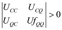 .
.
Thus, this leads to the following:
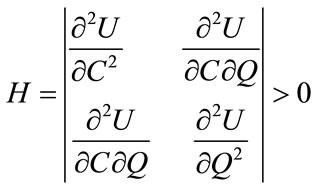 or
or 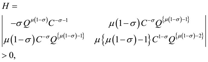
or![]() .
.
Then, we obtain the following restriction:
 .
.
Appendix 2: Derivation of (32)
We can rewrite Equation (22) as
Taking the derivative with respect to T, we have:

Arranging terms, we obtain the following:
 (22’)
(22’)
Taking the limit of Equation (29) as , we have:
 .
.
Thus, we have:
 (29’’)
Then, using Equations (7), (28) and (29’’), the above Equation (22’) leads to the following:
 (32)
(32)
Appendix 3: Proof of Proposition 1
Suppose that  holds true.
From Equation (31), we have:

This leads to the following:
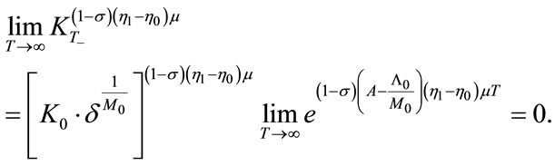
Taking the limit for T to infinity, Equation (32) leads to the following:
This implies that for infinitely large T, V(T) is not decreasing, meaning that:
 .
.
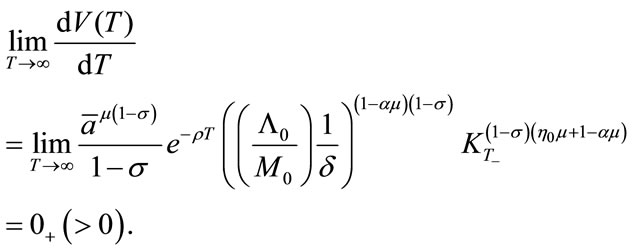
Appendix 4: Proof of Proposition 2
When  holds true,
Thus, Equation (32) indicates: .
.
Given this condition, if  holds true,
  must change its sign from positive to negative at least once as T increases. In other words, the conditions:
 , and
, and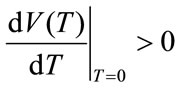 are sufficient for the existence of a finite optimal T, that is: 0 < T* < ∞.
Notice that the condition  has equivalent forms as follows:
or or
or or
or 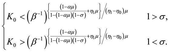
With these sufficiency conditions, the optimal T is yielded as a solution of the following:
 .
.
This is expressed as follows:
 or
or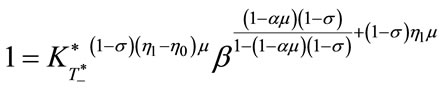 or
or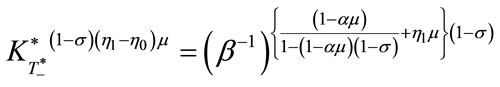 or
or .
.
To solve for T*, recall Equation (31), that is:
![]() or
or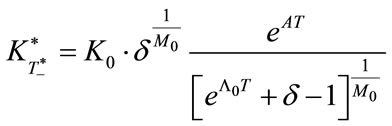 .
.
Then, we finally obtain Equation (36).
Appendix 5: Proof of Proposition 3
It is noted that when  and
and  hold true,
  approximates
 , that is:
 because:

With the approximations 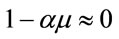 and
and , Equation (37) provides the following approximation:
 or
or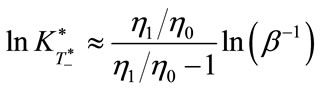 .
.
Taking derivatives for the both sides of the last equation with respect to  yields the following:
 or
or
 .
.
From Equation (36), considering that 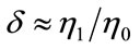 and T→∞, we have the following:
 or
or
 .
.
Again, taking the derivatives for the both sides of the last equation with respect to  yields the following:
 or
or .
.
Notice that the sign of the derivative is determined by the sign of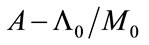 . Since we are assuming
  , the sign of
 , and that of
  are always same. Thus, (42) is evident.
Appendix 6: Summary of Cunha-e-Sá and Reis (2007)
This section summarizes the study of Cunha-e-Sá and Reis (2007).
Their model is described as follows:
 (A.1)
(A.1)
s.t. 

 .
.
υ, γ, and f represent the quality upgrade at T, the marginal cost of the technology adoption, and fixed costs, respectively. Other notations are the same with those of our study, presented in the article.
One of main differences between the model above and ours is the definition of environmental quality. Another difference is the existence of the last term (γυ + f) in (A. 1), representing the total cost of technology adoption.
The model leads to the value function as a function of T as follows:
 (A.2)
(A.2)
Examining the property of the value function, Cunhae-Sá and Reis addressed the following propositions:
Proposition 1
If δ < 1, then V(T) is increasing in T, and the country never adopts new technology, or, T* = ∞.
Proposition 2
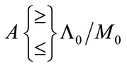
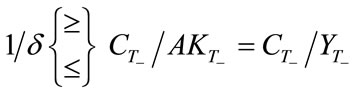
Let δ > 1. If (1) σ < 1, it is always better to adopt new technology within a finite period T than to never adopt it. In particular, it is optimal to adopt it immediately if , for T = 0. For (2) σ > 1, the country either adopts it immediately or never adopts it.
Proposition 3
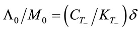
Given the results in Proposition 2, for δ > 1 and σ < 1, and 0 < T* < ∞, the capital level at the optimal timing of adoption is represented by the following:
 . (A. 3)
Proposition 4
For δ > 1, σ < 1, and 0 < T* < ∞ when technology adoption is anticipated, prior to its adoption, the growth of consumption and capital accelerates. Moreover, environmental quality decreases.
NOTES
1Brock and Taylor [12] and Bretschger and Smulders [13] provide comprehensive surveys on relationship between economic growth and the environment. Acemoglu et al. [14] introduce an advanced concept regarding technology called “directed technological change” and apply it to the growth with environmental constraints.
2Brock We do not explicitly consider the case of ( =1 in this paper. It is well-known that the utility function defined in this way approaches log(CQμ) as ( (1. Thus, our analysis implicitly includes the case of ( =1 as a limit. To explicitly include the case in our analysis, we need to repeat the same mathematics for the logarithmic utility function. Such simple repetition of analysis would not produce any additional implications while it makes our mathematical description double. It is left to the readers.
3These restrictions are conditions such that the Hessian matrix for the utility function is negative definite for all Ct and Qt. For the detail, see Appendix 1.
4Brock Notice that δ is defined as (30). It approximates unity when the difference between η0 and η1 is very small (i.e. η0 ≈ η1) and the utility function is close to logarithmic one (σ ≈ 1).