Journal of Environmental Protection
Vol. 4 No. 1 (2013) , Article ID: 27172 , 14 pages DOI:10.4236/jep.2013.41002
The Geochemistry of Heavy Metals in the Mudflat of Salinas de San Pedro Lagoon, California, USA
![]()
1Geosciences and Environment Department, California State University, Los Angeles, USA; 2Scripps Institute of Oceanography, University of California, La Jolla, USA.
Email: *mrezaie@calstatela.edu
Received October 1st, 2012; revised November 2nd, 2012; accepted December 4th, 2012
Keywords: Salinas De San Pedro; Bioavailability; Heavy Metal; Geo-Accumulation Index; Enrichment Factor; Lagoon Water Pollution
ABSTRACT
Sediment core samples were collected from the Salinas de San Pedro to assess the pollutant deposition processes in response to extensive human activities. Analysis of the sediment samples for heavy metals and some trace elements was conducted with ICP-OES for 20 sites showing enrichment for some of trace and heavy metals. The results demonstrated that heavy metal concentrations in mud varied greatly for each metal, with concentration values (mg/g) ranging from 1.05 - 4.8 (Al); 0.003 - 0.011(As); 0.001 - 0.005 (Cd); 0.02 to 0.82 (Cr); 0.085 - 0.47 (Cu); 5.98 - 14.22 (Fe); 0.06 - 0.19 (Mn); 0.03 - 0.67 (Ni); 0.05 - 0.38 (Pb); <0.008 - 0.069 (Se); 0.18 - 0.63 (Ti); 0.040 - 0.091 (V) and 0.149 - 0.336 (Zn). The Index of Geo-accumulation factor showed highest values for Pb, Mn, As, and Cu. Enrichment factors >1 for these elements suggest anthropogenic inputs for most metals. The bioavailability of metals in lagoon sediments has the potential to be highly dynamic with local waste and natural H2S discharge from existing fault line.
1. Introduction
Lagoons, estuarine, and coastal wetlands are complex and important ecosystems in which pollutant retention, sediment deposition, and fresh water-sea water interaction, occurs [1]. Highly populated urban areas (such as San Pedro, California) is almost always lead to the habitat, coastal marine life, and resources loss due to public access [2]. The behavior of metals in aquatic systems in such coastal environment is more popular due to the global anthropogenic alteration of trace metal cycles [3,4]. Aquatic animals are exposed to trace and heavy metals [5]. Therefore, sediment analysis is a good proxy for the assessment of the “geochemical status” and “environmental quality” in such environment [6]. Anthropogenic metals introduced into the aquatic environment often occur in two forms either in particulate or rapidly sorbed to particles [7,8]. In latter form, they contribute to the pool of metals linked with either suspended particulate matter within the water column or are finally built-in into deposited sediments [9]. It is widely recognized that behavior, transport, and fate of metals in aquatic systems are determined by nature of their association with solid substrate and/or organic material. The geochemical nature of such aquatic particles (e.g., sediments) determines the presence and form of trace metals in a lagoon environment. As a result, the geochemical association interferes with the uptake capability of an organism. Therefore, the process dictates the subset of metals that are available in free ionic form versus bond to particulate/sediment material from which they can be released.
Uptakes of metals by organism are also influenced by geochemical factors. These factors influences trace metal behaviors, which stems from increased flux of trace metals from terrestrials and atmospheric sources [10] to the aquatic environment due to human activities. For organisms that ingest either deposited sediments or suspended particulate matter as a food source, these anthropogenic metals may cause severe adverse effects and potentially leading to bioaccumulation by the organism and transfer via the food-chain to higher trophic levels [9]. The accessibility of anthropogenic metals to lagoon and estuarine organisms is reliant on the occurrence of the trace metal (exposure) and the nature of the geochemical component with which the trace metal is linked [11].
The most important geochemical components considered to influence the bioavailability of metals to sediment ingesting organisms is organic matter, Fe oxides, and Mn oxides [5,10-12]. For example, Rule and Alden, 1996 [13]; Thomas and Bendell-Young, 1998 [14] demonstrated under both laboratory and field conditions, that the accumulation of Cd by Macoma Balthica was best related to Cd associated with the easily reducible fraction of sediment (i.e. Mn oxyhydroxides).
According to Campbell and Tiessier (1989) [11] yet, the majority of studies directed at understanding the fate of metals in aquatic systems have paid attention primarily to the geochemistry of recently deposited sediments and the potential role of deposited sediments (DS) in providing a conduit for the transfer of metals from the sediment to sediment ingesting organisms. Nevertheless, due to their direct interface with the water, high surface area to volume ratio, and high nutritive quality [15] suspended particulate matter (SPM) may represent an ignored and perhaps further chemically and biologically relevant metal source for sediment ingesting organisms, as compared to DS. While marine sediments naturally retain different quantities of metals, any measurement of total heavy metal concentration as a criterion to judge metal contamination in the sediment environment is not reasonable to discriminate natural from anthropogenic sources. As a result the evaluation of an “Enrichment Factor” (EF) and/or “Contamination Factor” (CF) and “index of geo-accumulation” based on background values overcome this difficulty giving a simple quantitative measure for characterizing the sediment according to the degree of metal pollution [16].
Thus, identification of geochemical processes is the key for understanding the behavior, association, and distribution of metals in the geological and biological system of Salinas de San Pedro in California. This research study has focused on characterizing the SPMs and DS and their geochemical features in a local salt marshSalinas de San Pedro, CA, where such material provides food to a wide range of aquatic invertebrates.
Metals are associated with particulate transport and their disposal through lagoon is a function of hydraulic condition. Hydraulic condition by flood and ebb in San Pedro Salinas controls sorting and mixing processes, where contaminated and uncontaminated sediments are added to the lagoon’s storage and deposition. In this study, we quantified trace and heavy metal concentrations in DS and identified potential enrichment factor (EF), contamination factor (CF), and index of geoaccumulation (Igeo) patterns for a set of trace and heavy metals and their origins.
In summary, the purpose of our work is to a) quantify origin and degree of heavy metal and trace elements pollution and to develop sediment pollutants base-line data for Salinas de San Pedro as a unique habitat; b) characterize the geochemistry of deposited sediment within lagoon environment over a one-year period in low tide level; c) understand the factors which determine metal mobility in intertidal mud flat; d) Evaluate the role of H2S gas discharge from local active faults on the enrichment of metals in very fine particulate in water and its importance for the bioavailability of metals in anoxic sediments environment. This study is first to link the metal enrichment in mud and the role of naturally discharged H2S gas in salt marsh sediments on and/or near active earthquake fault line in southern California.
2. Materials and Methods
2.1. Study Location
The Salinas de San Pedro is located in Long Beach, California, USA. The mudflat habitat provides an interesting case study in metal geochemistry in a system with a high suspended particulate concentration through ebb (low tide) and flood (high tide). Salinas de San Pedro is an anthropogenically impacted and entirely manmade salt marsh lagoon, which is also a critical habitat for many sensitive species such as the benthic bivalves. Salinas de San Pedro was created by the Port of Los Angeles in 1985 to replace lost shallow-bottom fish habitat. The area is divided by habitats, representing the rocky shore (hard substratum), sandy beach and mudflat (soft shifting bottoms), and the open ocean. The study area is limited to the 3.75 acre (15,175 m2) salt marsh mudflat and its habitat (Figure 1). The depth of water changes from 1m along the shore area to 2 m in the central part.
The San Pedro salt marsh environment hosts distinct communities of plants and animals, which have evolved characteristics such as adaptations that enable them to reside there [17,18]. According to the latter web site the main food pathway in the mudflat is through the bacterial breakdown and decay of plant material such as eel grass to yield organic debris. The detritus material is used by a large variety of invertebrates, which in turn are eaten by fish and birds. The plants along the shore provide resting sites and food sources for many of the animals living in a mudflat. Natural factors affecting the Salinas de San Pedro like other wetlands include storms that flush the system, temporarily changing the balance between fresh and salt water [18]. The Salinas is nourished daily by the tides and seasonally by storm drain runoff. It is considered as “nurseries of the sea”, providing a protective nutrient-rich habitat for baby fish. In other words, many outer coast and offshore fish species are dependent upon these types of estuaries as breeding or nursery grounds for their young. Additionally, more than half of local commercial and sport-fish species spend some time in a mudflat or other wetland habitat. Besides, the Salinas de San Pedro traps sediment nutrients and pollution of the local storm drainage runoffs as well as absorb excess
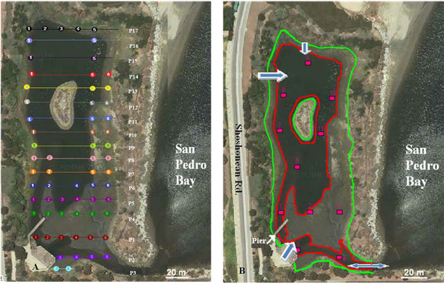
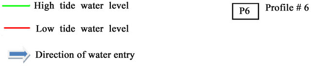
Figure 1. Map of sampling and study location (adapted from Google Earth, 2012); (a) Core-depth integrated composite samples 0 - 20 cm using hand core sampler; (b) Scoops and grab samples from mudflat surface (from top 2 to 4 centimeters).
polluted water that flows toward the ocean from Cabrillo Marine Aquarium excess waste water and storm drains.
The sampling stations are presented in Figure 1. All sampling were conducted in Lowest Low Tide Water (LLTW). The total of 17 profiles was identified in 3.75 acre of salt marsh. Up to six samples were taken in six evenly spaced locations (10 m apart).
According to EPA sediment sampling guideline and method [19] two types of samples were collected: a) Core samples: depth integrated composite samples 1 - 20 cm using hand core to understand vertical record of contamination (Figures 1(a) and (b)) Scoops or surface sediment (top two to four centimeters) grab samples (Figure 1(b)). This type of sampling is appropriate for benthic, sediment oxygen demand (in situ), recent ambient conditions, and recent contaminant investigation and grain size analysis. Eleven scoops surface samples were grabbed using hand shovel cylinder. A hand core (AMS Soft Sediment Core Sampler) was used as core sampling device to collect samples at depth of 20 cm below surface. Each sample was split in 2 samples from 1 - 10 cm and 10 - 20 cm respectively.
2.2. Parameter Selection
Each sample was analyzed on many parameters selectively based on the purpose of our study, the data quality objectives, and resource availability. All analyses were conformed to SW-846, 40 CFR Part 136, EPA Manual, Surveillance Methods and Quality Assurance Practices, or Standard Methods as appropriate [20].The chemical analysis including organic matter (OM), metals analysis (Ag, As, Cd, Cr, Cu, Fe, Mn, Ni, Pb, Se, Sr, Ti, V, and Zn) using ICP-OES. Physio-chemical analysis are conducted for particle size, appearance/texture/odor/color. Other data collection including overlying water quality including: water temperature, water depth, dissolved oxygen (DO), biological oxygen demand (BOD), conductivity, pH, water turbidity in ebb and flood condition in the Salinas de San Pedro.
Organic Matter (OM) was measured in un-sieved sediment as follows: 1 g of dry sample was heated at 450˚C in porcelain crucibles for 12 hrs. OM was combusted to ash and carbon dioxide at this temperature. The weight loss (the Loss of Ignition) was considered proportional to the amount of organic carbon contained in the sample [21].
2.2.1. Quality Assurance (QA) and Quality Control (QC) of Analysis
According to EPA (1991) [20] QA were conducted to find out about the number of samples, variance, difference of means, and to evaluate field duplicates/ station replicates and criteria for acceptance of data. According to EPA the replicate samples are a complete separate collection of a sample at one site, which were collected for sample location one at Profile 1. Blanks/Field Duplicate samples were collected for the purpose of QC and QA. Field blanks are samples of uncontaminated silica sand collected using the same sampling equipment and techniques as the sediment sample collections. According to EPA guideline (2001) [20] 10% of the sediment samples were collected as duplicates and 5% as blanks or equipment rinses. Field duplicate samples are collected to determine laboratory analytical variability and/or field compositing techniques and of sediment heterogeneity within a single collected sample. Duplicates are collected by “splitting” a sample that has already been collected into two identical samples for analysis. BH1-1 and BH1-2 were run twice (a, b), thus summing six replicates for ICP analysis. Some samples e.g. BH3-3 had enough material for only one replicate. Equipment rinse samples for sediment samples are comprised of a distilled and deionized water rinse following equipment decontamination. The equipment rinse samples and field blank samples are used to demonstrate that significant amounts of contaminants are not introduced into the sediment samples from sampling equipment or sample handling [22].
All sampling equipments were cleaned and decontaminated (acid washed with nitric acid 1N) before sampling. Sample containers (Teflon®) were placed in clear plastic bags to minimize cross-contamination of the shipping container and to protect laboratory personnel. Before each sampling period, sample containers were labeled with the site name, date, time of collection, and the name of the sample collector and/or other information specified by the laboratory [23]. Following each sampling period, sediment samples were chilled and stored in coolers at 4˚C. A chain of custody form was accompanied each sample shipment.
Temperature and pH of the Salinas lagoon water were obtained using pH-meter (Accumet AP71) probe on a 2-point calibration. DO and salinity were measured in the field using handheld dissolved oxygen instrument (YSI 550A). All instruments including pH-meter and YSI were calibrated before using in the field. BOD was measured semi quantitatively in relationship to oxygen level. The ICP-OES instrument, available at the Analytical Facility of the Scripps Institution of Oceanography, UCSD was calibrated before every run by successive dilution of a 100 µg/g multi-element instrument calibration standard solution (Fisher Scientific, CA, USA). Recovery of the QA standards was analyzed every sample over the course of the run was 103%, while internal blanks were analyzed to assess any background contamination originating from the sample manipulation was negligible.
2.2.2. Grain Size Analysis
According to ASTM D 422 [24] standard test method for particle size analysis of Salinas de San Pedro was conducted using dry and wet methods. Eleven collected bulk (scoop) samples were tested first for grain size analysis. A representative oven dried sample (about 50 g) was chosen for grain size analysis. The percentage of soil retained on each sieve was calculated on the basis of total weight of soil sample taken; then cumulative percentage of soil retained on successive sieve is found. Later, the graph constructed for log sieve size data vs. % finer fraction corresponding to 10%, 30% and 60% finer. The obtain diameters from graph are D10, D30, D60.
The grains smaller than 1/16 mm in diameter were analyzed using SediGraph® III 5120 (Micrometrics Inc.), which measures the gravity-induced settling rates of different size particles in a liquid with known properties. This is an extremely effective technique for providing particle size information for a wide variety of very fine materials. The SediGraph® instrument, available at the Sedimentology Lab, Cal State LA was calibrated before every run by using calibration standard solution.
2.2.3. Trace and Heavy Metal Analysis
For determination of trace elements [25], sediments freshly collected were dried at 70˚C for several days before being homogeneously crushed in a silicon mortar and the 63 µm fraction separated by dry sieving. A small amount (about 0.2 g) of that fraction of sediment was weighed using a Sartorius CP225D analytical microscale (Data Weighting Systems, IL, USA) connected to a notebook computer for accurate recording of measurements. Sediment samples were digested using a mixture of HCl:HNO3 (3:1) at using 80˚C using a Ethos EZ microwave (Milestones, CT, USA) for analysis of Ag, Al, As, Cd, Cr, Cu, Fe, Mn, Ni, Pb, Se, Sr, Ti, V, and Zn [25]. The digested sample solutions were analyzed using Inductively Coupled Plasma Optical Emission spectrometry (ICP-OES) 3000 XL with detection limits ranging from 0.05 × 10⁻⁶ to 4.0 × 10⁻⁶ mg×g−1 depending on the element (Perkin Elmer, CA, USA). QA and QC were assessed using duplicates, method blanks and standard reference materials according to EPA standard.
2.2.4 Enrichment Factor (EF)
Since trace metals occur naturally in the earth’s crust, it cannot be assumed that an environment is automatically anthropogenically contaminated when trace metals are found in its sediments. We utilized the EF method, a widely used normalizing measure, to distinguish between natural and anthropogenic metal sources [26-29]. In EF calculation, Al was used as earth crust value by Turekian and Wedepohl, (1961) [30]. Similarly, Fe was used as a normalizing factor by Ergin et al. [31] and Szefer et al. [32]. We used in Fe as normalizing factor this study. Thus, EF is defined as:

where Csample is trace element concentration in the sample, Ccrust is trace element concentration in the continental crust, Fesample is Fe content in the sample, and Fecrust is Fe content in the continental crust [33] (Taylor and McLennan, 1995). We then used criteria set by Birth (2003) [34] to score the severity of the EFs, in which EF < 1 is equal to no enrichment, 1 - 3 is minor enrichment, 3 - 5 is moderate enrichment, 5 - 10 is moderately severe enrichment, 10 - 25 is severe enrichment, 25 - 50 is very severe enrichment, and >50 is extremely severe enrichment.
2.2.5. Contamination Factor (CF)
The level of contamination of sediment by a metal is often expressed in terms of a CF:
A concentration factor, calculated as the ratio between the metal content at a given sediment sample and the normal concentration levels. This will reflect the metal enrichment in the sediment when CF > 1 for a particular metal, it means that the sediment is contaminated by the element, and if CF < 1, then there is no metal or low contamination by natural or anthropogenic inputs. We used 1 ≤ CF ≤ 3 for moderate contamination, 3 ≤ CF ≤ 6 for considerable contamination, and CF > 6 for very high contamination. While calculating the CF of the sediments in the study area, we have taken the world crustal average contamination of the trace metals under consideration reported by of background values.
2.2.6. Index of Geo-Accumulation (Igeo)
The assessment of sediments enrichment with elements can be carried out in many ways. The most common ones are the Igeo and EFs. A quantitative measure of metal pollution in aquatic sediments was introduced by [35], which is called the “index of geo-accumulation”. Numerous researches have employed it to assess the contamination of soils and sediments. It determines contamination by comparing current metal contents with pre-industrial levels. The content accepted as background is multiplied each time by the constant 1.5 in order to take into account natural fluctuations of a given substance in the environment as well as very small anthropogenic influences. The index of geo-accumulation provides a simple and quick method to determine the “extent of pollution” in a lake or river bed sediment by means of the trace element load in sediments above background values, but it does not give further information to the mobilization and bioavailability of the trace element [36]. The Igeo value reflects the degree of contamination of the sediments by a metal [33]. The value of the Geo-accumulation index is described by the following equation:
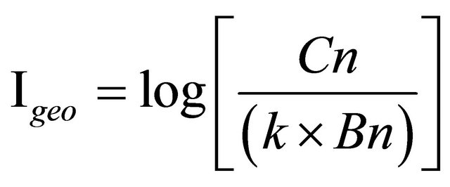
Cn: metal content in tested sediment/soil, Bn: background content; here the average metal content in the earth crust of (×) mg/kg k = 1.5, to consider possible variations in the background data due to lithogenic effects (constant factor).
According to [33] (Taylor and McLennan, 1995) the interpretation of the obtained results is as follows in which, Igeo ≤ 0 is practically uncontaminated, 0 < Igeo < 1 is uncontaminated to moderately contaminated, 1 < Igeo < 2 moderately contaminated, 2 < Igeo < 3 moderately to heavily contaminated, 3 < Igeo < 4 heavily contaminated, 4 < Igeo < 5 heavily to very heavily contaminated, and Igeo ≥ 5 very heavily contaminated.
2.2.7. Salinas de San Pedro and Palos Verdes Fault (PVF)
The Palos Verdes fault is an active geologic structure along the western margin of the Los Angeles basin and Inner Continental Borderland. Reflection seismic analysis and investigation conducted by [37] Shaw (2007) indicates that a rupture on the segment of the PV fault extends from the San Pedro Shelf across Long Beach harbor. Onshore, the earthquake faults such as Palos Verdes fault bounds the eastern margin of the uplifted Palos Verdes Hills, and extends offshore at the Port of Los Angeles southwestward into San Pedro Bay. Salinas de San Pedro located on SE segment of the fault (Figure 2). Local seismic activities in southern CA may cause forming cracks and fractures allowing large amounts of trapped gas leak upward along the fault line. In the same way H2S gas seeping from the ground at Salinas de San Pedro likely derived from geologic formation, which holds oil and other hydrocarbon beneath the lagoon. High concentrations of H2S in soil can kill the roots of trees and brushes and causes anoxic environment. Besides, H2S gas is heavier than air; and when it leaks from the mud, it can collect in mudflat, posing a potential danger to species and enrichment of some metals by formation of metal sulfide (Figure 2).
3. Results
Lagoon Sediment Characteristics
Grain size distribution for all bulk samples were shown in Figure 3. The bulk or grab samples showed mud as an overall distribution pattern in Salinas de San Pedro on the lagoon surface. The bulk samples also suggest an impor-

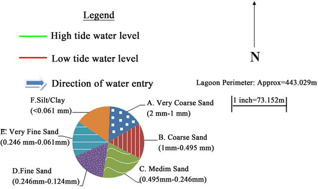
Figure 2. Lagoon sediment characteristics and distribution.
tant contribution of terrigenos material originating from runoff of surrounding lagoon. On the west side of lagoon the grain size was dominated by “fine sand” and “very fine sand”. The amount of clay were increased from SW to NW of lagoon (samples 1, 6, 7 and 8). On the east side, the “medium sand” was dominant grain size, yet the sample 10 in NE side showed the highest clay and silt content. The samples 9 and 2 in north and south side of lagoon showed the medium sand as highest percentile. It seems that the flood and ebb condition has deposited the “medium and course sand” on the east side and left the fine to very fine particles (silt and clay) on the west side. Near the runoff places were the medium and fine sand dominant grain size (Figure 2).
Overall, sediment samples was greenish grey to brownish color with rust stains and change in color from lighter to darker in the core samples. Sediment samples had “rotten egg” and very oily smell. Bioclast were present in most samples. Salt grass and pickle weed grow along the banks of this wildlife refuge. Moreover, the numerous holes on the mud surface are the evidence of the thriving underground community of invertebrates that dominate the lagoon’s mud. Overall, the Salinas de San Pedro contains mainly fine silt/clay material with high LOI level (Los of Ignition [%]). The grain size analysis of fine grained core samples (<1/16 mm in diameter) revealed that the silt and clay in sample may. The physiochemical parameters were measured for 10 sampling locations in Salinas de San Pedro in Summer 2009. The result show extreme low DO level (mg/l) for L2 (2.10), L4 (1.84), L6 (3.7) and L8 (1.80), which correlates with the hydrogen sulfide discharge locations (Table 1). The extremely low oxygen level for L2, L4, L6, and L8 correlate with the locations of hydrogen sulfide. The presence of H2S gas is being discharged from local fault line could naturally increase the organic matter (OM). If too much OM is available, the existing oxygen supplies will be used up. As microorganisms decompose OM through respiration, they use up all available oxygen (Table 1 and Figure 2(b)). A semi quantitative analysis of BOD showed that L3, L4, and L8 had extremely higher BOD in compare to other locations. The pH has not changed within lagoon for the 10 sampling location. The water temperature in lagoon has changed from 17.5˚C to 19˚C during sampling period in summer (Table 1 and Figure 2(b)). Average salinity (‰) of lagoon water was recorded lowest for L7 (22) L8 (24) and L9 (28) due to dilution process next to the street runoff discharge locations in northern part of lagoon. The average salinity of water in other parts of lagoon showed a range of 32 - 34.50 (‰) a much closer values to average ocean water salinity in San Pedro Bay, southern California (Table 1 and Figure 1(b)). Twenty samples were taken from Salinas de San Pedro to measure the concentration of several heavy and trace metals. In general, heavy and trace metals appeared to be spread homogeneously throughout the lagoon, sometimes reaching higher levels in various sites, and most often mainly concentrated in fine grained sediments. Trace metal concentrations in the upper sediment core material and bottom sediments in the different sampling campaigns are displayed in the Table 2. Even though consist of ilite, montmorilonite, and smectite (Figure 3).
Mean value for Fe, Al, Ni, Mn, and Zn were highest among the others. In order to under standing these results, metal concentrations are compared to the (National Oceanic and Atmospheric Administration) NOAA-Marine Sediment Quality Guideline values [38], which designnates an Effects Range Low (ERL). Among samples, BH3-4 showed the highest concentration for Cu (0.47 mg/g), BH3-1 for Ni (0.67 mg/g, BH6-2 for Pb (0.38 mg/g), and BH-1 for Zn (0.34 mg/g) in southern section of Salinas. These values all exceeded the NOAA-ERL values (Table 2). The values showed overall a decrease toward the centre part of lagoon. Box-Plot (Figure 4) shows trace metal distribution in Salinas de San Pedro. A noticeable decrease in Cr, Cu, Mn, and Pb was observed when comparing concentrations in the surface layers of the sediment with those found in the bottom (10 - 20 cm). On the contrary, metals with higher attraction to OM (i.e. Cu and Zn) followed a scattered variation with overall higher concentration.
Several trace metals showed medium to high correlations within and between sample types. Biogenic metals (i.e. Cd, Co, Cu, Ni, Pb and Zn) are normally associated to OM as it is their main carrier phase. There is a good
Table 1. The physio-chemical parameters for 10 sampling locations in Salinas de San Pedro measured in Summer 2009.
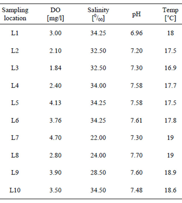
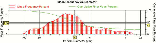
Figure 3. Diagram shows a representative lagoon sediment core samples (<1/16 mm in diameter) grain size characteristic and distribution conducted by SediGraph.
Table 2. Concentrations of several trace metals for 20 samples were taken from San Pedro Lagoon. NP= not processed. For Al, mean values with NP, indicate that the metal was in saturation in the liquid; *NOAA ERL value after (NOAA.gov) MCl= Max contam.
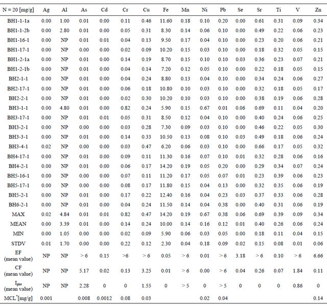
Table 3. Chemical species of heavy metals in soil with respect to solubility (modified after Fliep, 1998)[49] M = metal ion.


Figure 4. Box-Plot of trace metal distribution in Salinas de San Pedro.
correlation between Ti-Fe, Pb-Zn, Pb-Fe, Pb-Zn, and Pb-As for the sediments of the Salinas de San Pedro (Figure 5). The metal concentrations are strongly correlated to the iron and aluminium concentration. According to [39] Sheikholeslami et al. (2002), Al and Fe are a good proxy for terrigenous material and the amount of fine grained material in lagoon present. Fairly minor EF was prevalent for Cd, Fe, and Ni in the north and south section of lagoon just adjacent to waste water discharge. Cu and Ti also showed moderate EF values (ranges 3 to 5) in the south and northern lagoon during the ebb period.
Se and Zn showed moderate to high EF factor of 5 in the most samples but increased to severe EF values of the ranges 1 to >6 in the southern part of lagoon during the ebb period. Enrichment factors of As, Cr, Mn, Pb, Sr, and V showed extremely severe EF values (>6) in the central and south and northern part of lagoon. Overall, extremely severe EF values of very contaminated (>6) were predominant in most samples. Pb showed moderately to severe EF in the ranges of >3 to >6 respectively. EF values of As and Cr increased towards the discharge locations (hot spots), indicating a positive trend. The EF values showed an increase in contamination (highest; EF > 6) from the Cabrillo Marine Aquarium discharge location (samples from Profile 1) BH1,BH2, BH3 samples and from Profile 2) BH1, BH2, BH4, BH5 samples in southern shore as well as from street run off from Profile (17) BH1, BH2, BH3, BH4, BH5, BH3 samples. These samples were taken from discharge location areas. Other samples showed lower EF as the sampling locations are further away from discharge locations (Figure 1(b)). We expected a low EF for Fe due to its role as a reference element in sample and earth’s crust (Table 2).
The borehole (BH) sample from Profile (1) BH1,BH2, BH3 and from Profile (2) BH1, BH2, BH4, BH5 as well as street run off from Profile (17) BH1, BH2, BH3, BH4, BH5, and BH3 showed higher CF. These samples were taken exactly in discharge locations and their vicinities showed the highest CF (Figure 1(b)). The CF for the trace metals Cd, Ni, Se, Sr, Ti, and Zn in the core sediment of the Salinas de San Pedro are presented in Table 2, indicating a low to moderate level contamination of the sediments by these trace metals.
Mean CF rankings of core sediments samples were in As > Cd > Cr > Cu > Fe> Mn > Pb > Se > Sr > Ti >V > Zn. The CF value for As, and V lies in the ranges 1 to 3 indicating a moderate level of contamination by this metal. CF values for Cu (1.19 - 6.62; mean 3.25) was evident in the southern part of lagoon with a progressive increase of CF values ≥ 3 for the samples near discharge areas. The CF value for As (2.5 - 10), Mn (49 - 157) and Pb (255 - 1927) indicating a considerable to very high level of contamination by this metal. CF values for Pb and Mn were evident in the areas of waste water and H2S discharge (Table 2).
The Igeo for the trace metals As, Cd, Cr, Cu, Fe, Mn, Ni, Pb, Se, Sr, Ti, V, and Zn in the core sediment of the Salinas de San Pedro are presented in Table 3, indicating a low to moderate level contamination of the sediments by these trace metals. Mean index of geo-accumulation rankings of core sediments samples were in Pb > Mn > As > Cu > V > Sr > Zn > Cr > Ti > Cd > Fe > Se >Ni. In general, the sites are uncontaminated to extremely contaminate with respect to trace metals. The results of Igeo values are shown in Table 3. From this classification criteria, all the sediments could be approximately categorized as practically unpolluted with Cd, Cr, Fe, Ni, Se, Sr, Ti, and Zn, (Igeo < 0 for each trace metal), and moderately

Figure 5. Several trace metals showed medium to high correlations within and between sample types. Biogenic metals (i.e. Cd, Co, Cu, Ni, Pb and Zn) are normally associated to organic matter (OM) as it is their main carrier phase.
polluted with V (Igeo value 0 to 2 for both trace metals), moderately to heavily polluted with As and Cu (Igeo value 0 to 3), and heavily to extremely polluted with Mn and Pb, (Igeo value 4 to 5 and >5), respectively. Several metals (As, Pb, Mn, Cu, and V) exhibit concentrations sufficiently high to exceed sediment quality guidelines.
4. Discussion
The objective of this study was to find the source, origin, and the degree of heavy metal and trace elements pollution in San Pedro lagoon. We characterized DS and SPM within lagoon environment in ebb condition. Furthermore, we focused on assessing the roll of H2S gas discharge from local active faults on the enrichment of metals in very fine particulate in lagoon water. Yet, the role of natural H2S in controlling the dissolved metal availability has not been widely investigated. This study is the first, which investigates H2S and its widespread occurrence in salt marsh sediments from local earthquake fault line in southern California. We also focused on its importance for the bioavailability of metals in anoxic sediment environment.
Scientific understanding of metal association and behaviors in aquatic systems is dependent upon geochemistry. The following flowchart describes the role of DS and SPM in the uptake of metals by organisms. This process is influenced by geochemical factors that can cause metals to be more or less bioavailable (Figure 6). In addition, we understand how species are at greatest risk to metal exposure via their diet in such environment. Therefore, the concentrations of heavy metals, the grain size distribution in various fractions, and the OM content in sediments samples of Salinas de San Pedro were investigated.
In order to evaluate anthropogenic influences on the sediments, recommended EF values as an assessment criterion. EF values in the ranges 0.5 to 1.5 suggested that the trace metals sources might be entirely from crustal materials or natural weathering process, while EF values > 1.5 suggested that a significant portion of trace metal was delivered from non-crustal materials or non-natural weathering processes [40]. Yongming (2006) [41] also divided the metal pollution in sediments into different categories based on EF values. If EF ≤ 2, it suggested deficiency to minimal metal enrichment, and if a value of EF was greater than 2, it suggested various degrees of metal enrichment. The mean EF rankings of core sediments samples were in Sr > Cr > Mn > Mn > As > Pb > V > Cu> Zn > Se > Cd > Ti > Fe> Ni.
Table 2 shows the EF values of As, Cu, Cr, Pb, Se, Mn, Sr, V, and Zn were >2, showing a moderately to high anthropogenic impact on the trace metal concentration levels in the lagoon. Therefore, it could be as-
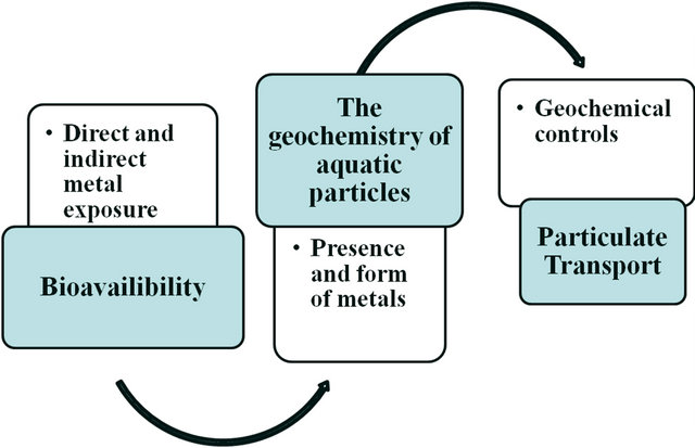
Figure 6. Flow chart of geochemistry of aquatic particles.
sumed that heavy metal and trace element pollution in the Salinas de San Pedro might entirely come from anthropogenic processes according to the scale proposed by Yongming et al. (2006) [41]. As a result, these trace metals pollutions should be currently a major concern. In addition, the EF values correlated with the significantly with samples contains sediments with finer fraction (very fine sand, silt, and clay). Geochemical properties of the fine sediment (DS and SPM) include particle size, organic content, concentrations of Fe and Mn oxides, total Cu, Pb and Zn concentrations, and the amounts of Cu, Pb and Zn partitioned onto organic matter and Fe and Mn oxides [12,15]. For instance, this information allows us to predict how sediment ingesting organisms are capable of exploiting sources of sediment as food resource.
According to geophysical investigation by Shaw (2007) [37], earthquake fault lines buried beneath the Salinas de San Pedro. These faults discharge hydrogen sulfide gas to the mudflat (Figure 2). This condition could naturally increase the easily reducible metals (Fe3+) and metal oxide (Fe2O3), organic matter (OM), and total metal (e.g. Cu, Pb, and Zn).
The Fe3+ and sulfate reductions are dominant electronaccepting processes [42] in the surface of Salinas de San Pedro sediments (0 - 20 cm). In other words, the H2S gas seeping through the fault from the ground at Salinas de San Pedro is likely derived Eh chemical reaction in anoxic environment.
As anthropogenic sources of contamination, we realized the boating area and Cabrillo Aquarium waste and sewage runoff is considered direct exposure. The presence of the dissolved metals in water may built organic complexes and be absorbed by particulate organic matter (Table 3). The dissolved particulate organic matter can flocculate or coagulate acting as a carrier for the trace metals to be digested [43]. Since metal sulfides are substantially less soluble in water, this promotes adsorption of HS− ions to the particle surface, contributing to a strong negative charge, which stabilizes the colloidal suspension. Therefore such material provides food to a wide range of aquatic invertebrates. A study by Karbanee et al. (2008) [44] showed that nickel sulfide precipitation was dependent on the availability of reactive sulfide species (i.e. HS−) in solution, which was in turn dependent on the pH of the solution. Due to the buffering characteristics of bicarbonate ions in seawater the pH of the water remained relatively unchanged between pH 6.9 and 7.6. (Table 2). More likely under these conditions, sulfide speciation equilibrium tends towards HS− ions [44,45] therefore metal ions precipitation may enhance. This implies that risks related to metal (such as Cd) uptake by organisms are relevant.
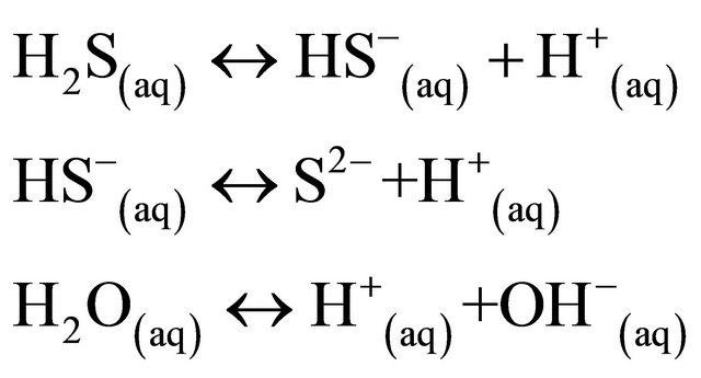
This reaction yields highly reactive hydrogen sulfide ( ), most of which diffuses upward and re-oxidized to
  by oxygenated ocean water in the surface sediment. This will precipitate Fe (II) in reducing sediment to yield iron mono sulfide. Andrews et al. (2004) [46] also demonstrate the same process with involving sulfate reducing bacteria, which metabolize organic matter.
Oxidizing conditions generally increase the retention capacity of metals in soil and sediments, while reducing conditions will generally lessen the retention capacity of metals [47]. Reducing conditions within mudflat also cause metal mobility, particularly of manganese and iron. The transition to oxidizing condition in ebb, solid iron oxide (e.g. FeOOH) will precipitate [46], dramatically, reducing the mobility of metals, which co-precipitate with iron. Vanbroekhoven et al. (2006) [48] demonstrate also that the transfer and the chemical stability of metal contaminants in soils and sediments are controlled by a complex series of biogeochemical processes depending on variables like pH, clay content, and redox potential. This relatively mild example illustrates the importance of redox conditions in contaminated lagoon water.
Toxic heavy metals and micronutrients utilized as metal ions exist in mud as species with several types of mobility and take part in many interactions. In liquid phase they exist as hydrated ions, soluble organic and inorganic complexes and as a component of fine disperse floating colloids. In the solid phase they occur as insoluble precipitates and minerals, on the surface of organic and inorganic colloids in exchangeable and non-exchangeable (specific adsorbed) forms (Table 3). The results showed that the iron concentration was decrease the bottom of the core sample (10 - 20 cm). Han et al. (2011) [42] also suggest that sulfides are very reactive components in the pore fluids with possible removal as metal sulfides, the main cause of the iron disappearance below 5 cm of core samples.
The effect of the flood water salinity on the mobility of heavy metals was investigated in similar research paper by Du Laing et al. (2008) [50] for intertidal sediments of the Scheldt estuary (Belgium). They monitored metal concentrations in pore water and surface water to study the potential effects of flood water salinity on metal bioavailability in duckweed (Lemna Minor). The results of the research by Du Laing et al. (2008) [50] showed that the salinity was found to primarily enhance the mobility of Cd and its uptake by duckweed. Furthermore, this research shows that Cd concentrations in pore water of soils and sediments significantly exceeded sanitation thresholds and quality standards during flooding of initially oxidized sediments. This implies that risks related to Cd uptake by organisms are relevant when constructing flooding areas in the brackish zones of estuaries. Du Laing et al. (2008) [50] also suggest that these risks can be reduced by inducing sulfide precipitation because Cd is then immobilized as sulfide and its mobility becomes independent of flood water salinity. This suggests that natural sulfide com-pounds in Salinas de San Pedro lagoon water may precipitate the heavy metals in pore water of silt and clay and thus being absorbed on the clay surface. This is possible by the interactions of these clay surfaces with water exchangeable cations.
5. Conclusions
This study has demonstrated that, Salinas de San Pedro sediments are geochemically distinct with respect to concentrations of Mn and Fe oxides, organic matter, and amounts of heavy and trace metals (As, Cu, Pb, Sr, Ti, and Zn). The results show higher concentrations of metals in the sediment samples during low tide (ebb) period near or at the H2S and waste discharge locations (hot spots) in Salinas de San Pedro. The latter samples had significantly higher reducible Fe and Mn content (possibly Fe and Mn oxide), higher organic content, and total metal concentrations than those of farther from hot spot locations. Metal bioavailability from DS (pre-existing SPM) near the fault line has the potential to be greater during ebb periods, where a greater proportion of the metal occurs in an easily reducible form (bioavailable) as compared to high tide. Furthermore, organisms that do exploit both food sources (DS and SPM) tend to filterfeed on solid organic matter during the periods of low tide. Hence, it is possible that filter-feeders consume contaminated suspended organic matter during both low and high tide where labile metals are at their greatest. We conclude that the most likely sources for these element enrichments (especially As, Cr, Pb, Se, Ti, and Zn) are naturally occurring H2S as well as intensive industrial activities in the local harbor during the last two decades. EFs calculation showed that anthropogenic activities to be the source of the contamination input in the Salinas de San Pedro. Such activities include those associated with the nearby Cabrillo waste water runoff in southern shore and also storm drains in northern shore of the lagoons. The boating activity and waste disposal probably also contribute to organic and inorganic contaminants in the lagoon. As a result, these trace and heavy metals pollutions in Salinas should be currently a major concern.
Under these circumstances, we suggest that the bioavailability of metals in lagoon sediments has the potential to be highly dynamic with natural H2S discharge from existing fault line and local waste discharge. The routes of metal uptake by filter-feeders and lagoon organism could be identified correctly with further studies of bivalves during low and high tide level.
6. Acknowledgements
The authors thank the Drs Latz-Deheyn Laboratory at Scripps Institution of Oceanography, UC, San Diego for sample preparation and ICP analysis and Dr. Ramirez at CSU, Los Angeles for using SediGraph and mud lab for grain size analysis. We thank also Cabrillo Marine Aquarium administration for allowing us to sample the Salinas de San Pedro mudflat.
REFERENCES
- J. Bai, et al., “Arsenic and Heavy Metal Pollution in Wetland Soils from Tidal Freshwater and Salt Marshes before and after the Flow-Sediment Regulation Regime in the Yellow River Delta, China,” Journal of Hydrology, Vol. 450-451, 2012, pp. 244-253. doi:10.1016/j.jhydrol.2012.05.006
- K. Schiff, et al., “Assessing Water Quality in Marine Protected Areas from Southern California, USA,” Marine Pollution Bulletin, Vol. 62, No. 12, 2011, pp. 2780-2786. doi:10.1016/j.marpolbul.2011.09.009
- U. Forstner and G. Wittman, “Metal Pollution in the Aquatic Environment,” 2nd Revised Edition, Springer Verlag, New York, 1981. doi:10.1007/978-3-642-69385-4
- W. Solomons and U. Forstner, “Metals in the Hydrocycle,” Springer-Verlag, New York, 1984, p. 349. doi:10.1007/978-3-642-69325-0
- S. N. Luorna, et al., “Determination of Selenium Bioavailability to a Benthic Particulate and Solute Pathways,” Environmental Science & Technology, Vol. 26, No. 3, 1992, pp. 485-491.
- European Commmision, “Establishing a Framework for Community Action in the Field of Water Policy. European Commission,” 2000.
- E. A. Jenne and J. M. Zachara, “Factors Influencing the Sorption of Metals,” In: K. L. Dickson, A. W. Maki and W. A. Brungs, Eds., Fate and Effects of Sediment-Bound Chemicals in Aquatic Systems, Pergammon Press, New York, 1987, pp. 83-98.
- P. Regnier and R. Wollast, “Distribution of Trace Metals in Suspended Matter of the Scheldt Estuary,” Marine Chemistry, Vol. 43, No. 1-4, 1993, pp. 3-19.
- J. R. Pierre Stecko, “Contrasting the Geochemistry of Suspended Particulate Matter and Deposited Sediment of the Fraser River Estuary: Implication for Metal Exposure and Uptake in Estuarine Deposit and Filter Feeder,” Dissertation, 1992, p. 213.
- A. Tessier, et al., “Relationships between the Partitioning of Trace Metals in Sediments and Their Accumulation in the Tissues of the Freshwater Mollusc Elliptio Complanata in a Mining Area,” Canadian Journal of Fisheries and Aquatic Sciences, Vol. 41, No. 10, 1984, pp. 1463- 1472.
- P. G. C. Campbell and A. Tessier, “Geochemistry and Bioavailability of Trace Metals in Sediments,” In: A. Boudou and F. Ribeyre, Eds., Aquatic Ecotoxicology: Fundamental Concepts and Methodologies, Vol. 1, CRC Press, Boca Raton, 1989, pp. 125-148.
- L. Bendell-Young and H. H. Harvey, “Geochemistry of Mn and Fe in Lake Sediments in Relation to Lake Acidity,” Limnology and Oceanography, Vol. 37, No. 3, 1992, pp. 603-613. doi:10.4319/lo.1992.37.3.0603
- J. H. Rule and R. W. Alden, “Cadmium Bioavailability to Three Estuarine Animals in Relation to Geochemical Fractions of Sediments,” Archives of Environmental Contamination and Toxicology, Vol. 19, No. 6, 1996, pp. 878-885. doi:10.1007/BF01055054
- C. A. Thomas and L. I. Bendell-Young, “Linking the GeoChemistry of an Intertidal Region to Metal Bioavailability in the Filter-Feeding Bivalve Macoma Balthica,” Marine Ecology Progress Series, Vol. 173, 1998, pp. 197-213. doi:10.3354/meps173197
- J. R. Pierre Stecko and L. I. Bendell-Young, “Contrasting the Geochemistry of Suspended Particulate Matter and Deposited Sediments within an Estuary,” Applied Geochemistary, Vol. 15, No. 6, 2000, pp. 753-775.
- G. Adami, P. Barbieri and E. Reisenhofer, “An Improved Index for Monitoring Metal Pollutants in Surface Sediments,” Toxicology and Environmental Chemistry, Vol. 77, No. 3-4, 2000, pp. 189-197. doi:10.1080/02772240009358949
- M. Schaadt and E. Mastro, “San Pedro’s Cabrillo Beach,” Arcadia Publishing, Charleston, 2008, p. 128.
- Cabrillo Marine Aquarium Educational Handout, “Educators Guide to the Coastal Marine Environment,” 2000, p. 54.
- EPA, “Sediment Sampling Guide and Methodologies,” 2001, p. 35.
- EPA, “Ohio EPA Manual of Surveillance Methods and Quality Assurance Practices,” Division of Environmental Services, Columbus, 1991.
- W. E. Dean, “Determination of Carbonate and Organic Matter in Calcareous Sediments and Sedimentary Rocks by Loss on Ignition. Comparison with Other Methods,” Journal of Sedimentary Petrology, Vol. 44, No. 242, 1974, p. 248.
- M. A. MacKnight, “Handbook of Techniques for Aquatic Sediment Sampling,” Lewis Publishers, Chelsea, 1994.
- ASTM D 422, “Grain Size Distribution, Standard Test Method for Particle Size Analysis of Soils,” University of Texas at Arlington Geotechnical Engineering Laboratory, 2004, p. 7.
- ASTM, “Standard Guide for Collection, Storage, Characterization, and Manipulation of Sediments for Toxicological Testing,” ASTM Annual Book of Standards, Vol. 11, No. 4, 2004, pp. 1391-1394.
- D. D. Deheyn and M. I. Latz, “Bioavailability of Metals along a Contamination Gradient in San Diego Bay (California, USA),” Chemosphere, Vol. 63, No. 5, 2006, pp. 818-834. doi:10.1016/j.chemosphere.2005.07.066
- K. Selvaraj, V. R. Mohan and P. Szefer, “Evaluation of Metal Contamination in Coastal Sediments of the Bay of Bengal, India: Geochemical and Statistical Approaches,” Marine Pollution Bulletin, Vol. 49, No. 3, 2004, pp. 174- 185.
- J. Valdes, et al., “Distribution and Enrichment Evaluation of Heavy Metals in Mejillones Bay (23˚S), Northern Chile: Geochemical and Statistical Approach,” Marine Pollution Bulletin, Vol. 50, No. 12, 2005, pp. 1558-1568. doi:10.1016/j.marpolbul.2005.06.024
- C. W. Chen, et al., “Distribution and Accumulation of Heavy Metals in the Sediments of Kaohsiung Harbor, Taiwan,” Chemosphere, Vol. 66, No. 8, 2007, pp. 1431- 1440. doi:10.1016/j.chemosphere.2006.09.030
- K. Gnandi, et al., “Increased Bioavailability of Mercury in the Lagoons of Lomé, Togo: The Possible Role of Dredging,” AMBIO, Vol. 40, No. 1, 2010, pp. 26-42. doi:10.1007/s13280-010-0094-4
- K. K. Turekian and K. H. Wedepohl, “Distribution of the Elements in some Major Units of the Earth’s Crust,” Geological Society of America Bulletin, Vol. 72, No. 2, 1961, pp. 175-191. doi:10.1130/0016-7606(1961)72[175:DOTEIS]2.0.CO;2
- M. Ergin, et al., “Heavy Metal Concentrations in Surface Sediments from the Two Coastal Inlets (Golden Horn Estuary and Izmit Bay) of the Northeastern Sea of Marmara,” Chemical Geology, Vol. 91, No. 3, 1991, pp. 269- 285. doi:10.1016/0009-2541(91)90004-B
- P. Szefer, G. P. Glasby and A. Kusak, “Evaluation of the Anthropogenic Influx of Metallic Pollutants into Puck Bay, Southern Baltic,” Applied Geochemistry, Vol. 13, No. 3, 1998, pp. 293-304. doi:10.1016/S0883-2927(97)00098-X
- S. R. Taylor and S. M. McLennan, “The Geochemical Evolution of the Continental Crust,” Reviews of Geophysics, Vol. 33, No. 2, 1995, pp. 241-265
- G. Birth, “A Scheme for Assessing Human Impacts on Coastal Aquatic Environments Using Sediments,” In: C. D. Woodcofie and R. A. Furness, Eds., Coastal GIS, Wollongong University Papers in Center for Maritime Policy, Australia, 2003.
- G. Müller, “Chemical Decontamination of Dredged Materials, Combustion Residues, Soil and Other Materials Contaminated with Heavy Metals,” In: W. Wolf, J. Van deBrink and F. J. Colon, Eds., 2nd International TNO/ BMFT Conference on Contaminated Soil, Vol. 2, 1988, pp. 1439-1442.
- U. A. Förstner, C. Wolfgang and M. Kersten, “Sediment Criteria, Development,” In. D. Heling, P. Rothe and U. Förstner, Eds., Sediments and Environmental Geochemistry, Vol. 1, 1990, pp. 311-338. doi:10.1007/978-3-642-75097-7_18
- J. H. Shaw, “Subsurface Geometry and Segmentation of the Palos Verdes Fault and their Implications for Earthquake Hazards in Southern California,” Technical Report, National Earthquake Hazard Reduction Program Award, No. 6, 2007, p. 20.
- NOAA:Spo.Nos.Noaa.gov/projects/nsandt/sedimentquality.Html. 2009.
- M. R. Sheikholeslami and S. De Mora, “ASTP: Contaminant Screening Program; Final Report: Interpretation of Caspian Sea Sediment Data,” IAEA-Marine Environment Laboratory Internal Report, 2002.
- J. Zhang and C. L. Liu, “Riverine Composition and Estuarine Geochemistry of Particulate Metals in China— Weathering Features, Anthropogenic Impact and Chemical Fluxes,” Estuarine, Coastal and Shelf Science, Vol. 54, No. 6, 2002, pp. 1051-1070. doi:10.1006/ecss.2001.0879
- H. Yongming, et al., “Multivariate Analysis of Heavy Metal Contamination in Urban Dusts of Xi’an, Central China,” Science of the Total Environment, Vol. 355, No. 1-3, 2006, pp. 176-186.
- S. Han, A. Obraztsova, et al., “Sulfide and Iron Control on Mercury Speciation in Anoxic Estuarine Sediment Slurries,” Marine Chemistry, Vol. 111, No. 3-4, 2008, pp. 214-220. doi:10.1016/j.marchem.2008.05.002
- J. Santos-Echeandía, et al., “Metal Composition and Fluxes of Sinking Particles and Post-Depositional Transformation in a Ria Coastal System (NW Iberian Peninsula),” Marine Chemistry, Vol. 134-135, 2012, pp. 36-46. doi:10.1016/j.marchem.2012.02.006
- N. Karbanee, R. P. van Hill and R. P. Lewis, “Controlled Nickel Sulfide Precipitation Using Gaseous Hydrogen Sulfide,” Industrial & Engineering Chemistry Research, Vol. 47, No. 5, 2008, pp. 1596-1602. doi:10.1021/ie0711224
- T. P. Mokone, R. P. Van Hille and A. E. Lewis, “Metal Sulphides from Wastewater: Assessing the Impact of Supersaturation Control Strategies,” Water Research, Vol. 46, No. 7, 2012, pp. 2088-2100. doi:10.1016/j.watres.2012.01.027
- J. E. Andrews, et al., “An Introduction to Environmental Chemistary,” 2nd Edition, Blackwell Publishing, Oxford, 2004.
- J. E. McLean and B. E. Bledsoe, “Behavior of Metals is Soils,” USEPA Ground Water, 1992, pp. 1-25.
- K. Vanbroekhoven, et al., “Varying Redox Conditions Changes Metal Behavior Due to Microbial Activities,” Geophysical Research Abstracts, Vol. 8, 2006, p. 2292.
- G. Fliep, “Behavior and Fate of Pollutants in Soil,” In: G. Filep, Ed., Soil Pollution, Agricultural University of Debrecens, 1998, pp. 21-49.
- G. Du Laing, et al., “Effect of Salinity on Heavy Metal Mobility and Availability in Intertidal Sediments of the Scheldt Estuary,” Estuarine, Coastal and Shelf Science, Vol. 77, No. 4, 2008, pp. 589-602.
NOTES
*Corresponding author.