Journal of Environmental Protection
Vol. 3 No. 8A (2012) , Article ID: 21788 , 11 pages DOI:10.4236/jep.2012.328095
Monitoring Recreational Waters: How to Integrate Environmental Determinants
![]()
1Laboratory for Foodborne Zoonoses, Public Health Agency of Canada, Saint-Hyacinthe, Canada; 2Groupe de Recherche en Épidémiologie des Zoonoses et Santé Publique, Université de Montréal, Saint-Hyacinthe, Canada.
Email: patricia.turgeon@phac-aspc.gc.ca
Received June 7th, 2012; revised July 6th, 2012; accepted August 2nd, 2012
Keywords: Recreational waters; fecal pollution; environmental determinants; monitoring
ABSTRACT
Recreational waters are associated with a higher risk of disease for people engaged in activities that bring them into contact with these waters. The primary cause of contamination of recreational waters is fecal microorganisms, which may originate from various sources and involve several modulating factors, making it a complex public health and environmental issue. Monitoring recreational water quality should include two key components: Microbial water testing and monitoring environmental determinants associated with higher risks of contamination. Conducting both activities provides the foundation for a comprehensive assessment according to risk and the actual level of fecal pollution and thus could promote good management actions to ensure safe water quality. Nevertheless, monitoring of environmental determinants is rarely fully integrated in monitoring programs and is also harder to achieve, especially when water pollution is mainly associated with nonpoint sources. In order to achieve identification and monitoring of environmental determinants associated with fecal contamination of recreational waters, some specific steps should be followed and some questions must be answered. The objective of this review article is to present current knowledge on this topic and to suggest and discuss recommendations. Potential sources of contamination and factors able to modulate them should be identified and measured after the geographical area influencing fecal contamination of recreational water has been delineated. Statistical models have been developed to identify the relative importance of these environmental characteristics on fecal pollution of recreational waters but they do not allow for a full comprehension of the exact processes leading to this pollution, thus other methods should also be used to better understand these processes.
1. Introduction
In the last few years, health risks associated with activeties in recreational waters were a growing preoccupation for public health communities all around the world, but more specifically for industrialized countries. This interest can be explained in part by the growing attendance on public beaches, driven by climatic and demographic changes. In the next decades, global changes, including climate changes, will cause important perturbations to aquatic ecosystems. Among these, degradation of microbiological quality of surface waters is expected [1]. Climate changes will bring an increase in the frequency and intensity of rain events which will be followed by an increasing amount of water reaching watercourses by runoff [2]. This increased runoff will carry a larger amount of microorganisms. Moreover, the growing frequency of rain events could overload the sewer systems and the wastewater treatment plants, which were not designed to work with and treat this amount of water. These overloads could prevent the appropriate performance of treatment plants and thus lead to the dumping of wastewater directly into watercourses.
Human populations can be exposed to impaired surface water through drinking water but also through recreational waters. Different types of pollution can affect recreational waters, such as fecal contamination, cyanobacteria, and chemical pollutants. Fecal contamination can result in a large amount of microorganisms that lead to various types of illnesses including gastrointestinal illnesses (GI) and respiratory, skin, and ear infections [3]. GI illnesses are the most frequent diseases associated with activities in recreational waters but they are usually mild and self-limiting, which can lead to some difficulties in their monitoring. Nonetheless, epidemiological studies have shown positive associations between sporadic cases of GI illness and activities in recreational waters and between fecal contamination of these waters and GI outbreaks [4-8].
Surveillance of the microbial quality of recreational waters is mainly done by measuring levels of fecal microbial indicators such as Escherichia coli or fecal coliforms. This measurement can provide an indication of water quality relatively quickly, usually in 24 - 48 hours following the sampling. Different microbiological technologies like QPCR have been developed to palliate this time limit, providing results in only a few hours [9,10]. Moreover, predictive models have been elaborated from various meteorological parameters such as rainfall and wind speed in an attempt to predict the level of fecal contamination according to these conditions [11,12]. In general, these methods aim to answer the question: Are recreational waters safe for people today or in the next few days? Although these measures are crucial for quick decision making on the likelihood of a microbial hazard, they do not allow a complete evaluation of the risk of fecal contamination.
To account for a broader assessment of risk, the World Health Organization (WHO) recommends the evaluation and monitoring of sources of fecal contamination and environmental characteristics (environmental determinants) influencing this contamination in addition to water testing [13]. Unlike rainfall events and temperature, these characteristics are relatively stable in time and could explain as much as 40% of the fecal contamination variation for a beach [14]. Knowing and monitoring these determinants could help ascertain which beaches have a higher risk of fecal contamination. Integrating a sound assessment of both risk and determinants into the monitoring of fecal pollution using microbial indicators would provide the base for a more comprehensive and accurate evaluation and thus would promote good management actions to ensure safe water quality.
Monitoring of the sources of fecal contamination can be performed in different ways. The WHO recommends the annual census of every potential source of contamination of recreational waters by field inspection activities [13]. This precise and relevant method for point source pollution can be very difficult to apply to water bodies associated mostly with non-point source (diffuse) pollution, like most fresh and inland water bodies. Moreover, annual field campaigns can be time consuming and also very demanding in terms of financial and human resources, resulting in a big challenge when trying to apply them across large territories. Therefore, there is a need to develop new efficient methods able to characterize the proximal environment of beaches and thus contribute to the identification and monitoring of environmental characteristics associated with a higher risk of fecal contamination.
In order to achieve this identification and monitoring for recreational waters, some specific steps should be followed and some questions must be answered. The objective of this article is to conduct a review of knowledge on this topic and to suggest and discuss four steps that should be followed:
• Identify potential sources of fecal contamination of recreational waters.
• Identify factors able to modulate this pollution.
• Delineate geographical area influencing the fecal pollution of water bodies.
• Identify and apply methods for quantitatively measuring these sources and factors and assessing their association with fecal pollution of recreational waters in order to establish best monitoring practices.
2. Identify Potential Sources of Fecal Contamination of Recreational Waters
Sources of fecal contamination are various and can include urban, wildlife, and agricultural activities. Water contaminated by both animal and human sources of fecal microorganisms can represent a health risk for people engaged in recreational activities. Although it is assumed that, in general, animal sources of fecal contamination represent a smaller risk to human health than human sources [13], animals can carry zoonotic pathogens such as Salmonella, Campylobacter, and E. coli O157:H7, which may lead to gastrointestinal illness and sometimes severe sequelae [15,16]. Studies have indicated that risk of gastrointestinal illness associated with exposure to recreational waters impacted by animal feces may not be different from waters impacted by human sources. Nonetheless, human health risk from exposure to recreational waters impacted by non-human sources is still not well understood; some studies did not find statistically significant associations between illness risk and fecal contamination of water by animal sources [17,18].
2.1. Urban Activities
Urban fecal pollution can occur through different means. During rain events, waters can runoff by two major ways. They can reach watercourses via pluvial sewer systems, carrying many pollutants such as organic components and fecal pathogens coming from domestic wastes, domestic fauna, and wildlife [19]. Waters can also be directed to combined sewer systems that collect domestic industrial and pluvial waters [20]. However, during heavy rainfalls and rapid snow melts, water discharge coming into these systems can overwhelm wastewater treatment plant capacities and overload. Water containing pluvial waters and wastewater from domestic and industrial use can be discharged into watercourses by overload drains called combined sewer overflows (CSOs) [21]. CSOs may represent a health risk for people in contact with these waters since the principal source of bacteria it contains is from human waste, which can contain large quantities of fecal pathogens [22]. E. coli concentration associated with CSOs can reach more than 106/100ml, which it is much higher than recreational water guidelines [23]. Wastewater treated by wastewater treatment plants can also contain large amounts of fecal bacteria if these waters are not disinfected before being discharged into watercourses, placing people swimming in waters in close proximity to these discharges at higher risk for health problems [24].
Fecal pollution coming from urban activities and populations can also occur directly on the beaches. Bathers can be a source of fecal microorganisms via fecal accident, mainly where the proportion of children among bathers is high and if there are babies and toddlers in diapers [25,26]. Some outbreaks of Shigella sonnei (human pathogen) associated with activities in recreational freshwaters have been reported. In these outbreaks, the bacteria source mostly implicated were bathers who had been attending the beaches [27-29]. Bathers can also carry fecal microorganisms from the sand to the water and also stir up bottom sediment, making contact between bathers and the microorganisms trapped in sediment more frequent [30].
Domestic fauna such as dogs and cats can also be a source of fecal contamination. These animals can carry pathogens like species of Campylobacter, Salmonella, Giardia, and Cryptosporidium [31,32]. These microorganisms could reach watercourses mainly by runoff following rain events.
2.2. Wildlife
Wild animals can contribute to fecal pollution of recreational waters. Waterfowl have specifically been studied in the last decade [33,34]. These birds can be carriers of many fecal pathogens including species of Campylobacter, Salmonella, and Cryptosporidium and studies suggest they can be a source of contamination of recreational waters, particularly in rural regions [35-38]. Birds can pollute water by direct deposit of fecal material but also by contaminating the beach sand. Wild mammals can also carry fecal pathogens communicable to humans, although prevalence is usually low [39-41]. These animals can bring fecal microorganisms into watercourses by soil leaching and runoff during rain events and by direct deposit of fecal material.
2.3. Agricultural Activities
Agricultural activities can contribute to fecal pollution of waters and eventually recreational waters in many ways. Fecal pollution can come from animals and manure piles on farms and animal production sites. Livestock can carry and excrete in their feces zoonotic agents which may lead to various health problems from self-limiting GI disturbances to severe diseases that are potentially deadly. Zoonotic pathogens most often associated with farm animals are Salmonella Enterica, Campylobacter jejuni and coli, E. coli O157:H7, Giardia spp. and Cryptosporidium spp. [42,43]. These pathogens can reach watercourses mainly following rain events. Water contamination by stored manure on farms can result from leaking storage, overflows, or manure piles. A significant GI outbreak caused by E. coli O157:H7 and Campylobacter occurred in Walkerton, Canada in 2000 following a contamination of a municipal water well. Much of the evidence suggests that the origin of the contamination was runoff coming from a manure pile close to a cattle farm [44]. Manure spread on crop lands can also contain a large amount of fecal microorganisms [45]. As an example, fecal coliform concentrations measured in runoff waters following cattle manure spreading can reach 1.9 × 10⁴ to 1.1 × 10⁶/100ml, depending on the initial manure concentration [46]. Therefore, runoff waters coming from agricultural fields often exceed the drinking and microbiological guidelines for recreational waters [47]. Even if they can survive for many weeks on the soil after manure spreading, risk of water pollution by fecal microorganisms is highest soon after the spreading. On the other hand, some procedures can reduce the concentration of microorganisms in manure before spreading, such as aerobic or anaerobic digestion and composting [48,49].
In addition to manure spreading, animals at pasture can be responsible for water contamination through microorganisms present in their feces [50]. For instance, some agents can persist in soil for many months after exiting an animal’s gastrointestinal tract [51,52]. The impact of animals at pasture can vary according to animal density. A high density can lead to a large quantity of urine and feces on a relatively small surface, increasing the probability of nutrients and microorganisms reaching surface waters through runoff and also getting through the soil to reach the ground waters [53]. High animal density can also accelerate soil erosion which can increase runoff during rain events. The impact of animals at pasture could also be associated with their distribution across the watershed and if they have access to a watercourse [54].
3. Identify Factors Able to Modulate Fecal Pollution of Recreational Waters
Some factors can modulate fecal contamination of waters by influencing the passage of fecal microorganisms to surface waters, including vegetation, climatic conditions, soil type, and topography.
3.1. Vegetation
Riparian zones can reduce the concentration of fecal microbes coming from agricultural lands and entering surface waters by more than 90% by preventing soil erosion and contributing to absorption of runoff water [55-57]. However, no scientific consensus exists on the minimal required width for an efficient reduction of microorganism transfer, although it is known that recommended width is affected by ground slope and vegetation type [58]. Wetlands can capture many elements brought by runoff such as sediments, microorganisms, and nutrients, reducing water pollution [59,60]. According to a study carried out in an agricultural watershed, wetlands could capture as much as 68% of E. coli coming from runoff waters [60]. Forest areas can also be associated with better water quality given their capacity to reduce runoff, sediments, and nutrients in surface waters. They could also have a positive influence on surface water quality by promoting water infiltration to the water tables [61].
3.2. Climatic Conditions
Rain events and their intensity are an important factor affecting the transport of microorganisms at the soil level. Runoff can carry bacteria a long distance downstream and thus contribute to water pollution [62-64]. As an example, risk of fecal contamination of watercourses following manure spreading during dry periods would be significantly lower than when manure is spread within a few days before rain events [64]. If there is no rain during days following manure spreading, bacteria movement to watercourses will diminish and under some environmental conditions—UV rays and desiccation—bacteria count will also diminish [65]. Moreover, during rainfall some bacteria such as E. coli would be quickly carried away by runoff waters and would have less chance to interact with the soil matrix [66]. Furthermore, studies have shown positives associations between rain events and waterborne disease outbreaks [67-69].
Exposure to solar rays could also be an important element in the bacterial inactivation process in water and soil [62]. Bacteria count in water decreases more rapidly during sunny days than during cloudy days, even at various depths [70]. In general, microorganism survival is prolonged in cold temperatures [71].
3.3. Soil Type and Topography
The two major modes of microorganism movement with water in soil are the infiltration to ground waters and runoff to surface waters. Relative proportions of these two modes depend on various elements including the type of soil [72,73]. Soil composition such as clay and soils with high levels of organic matter can influence the movement and survival of microorganisms. High clay concentrations can influence this survival by offering a protection against environmental stresses such as UV and desiccation. For example, E. coli counts in soil could decrease more rapidly in sandy soil than in clay soil [74]. Humidity level can also influence the microorganism movement in soil. The higher the soil humidity, the more contaminated the runoff will be following a rain event because the high humidity facilitates microorganism transport to watercourses [63].
Land slope also plays a role in microorganism movement. The more steep the slope, the more runoff will occur and at faster speeds, which promotes soil erosion and particle movement, which includes microorganisms [62,73].
4. Delineate Geographical Area Influencing the Fecal Pollution of Water Bodies
There are two ways by which surface waters and eventually recreational waters can be fecally polluted: they can be contaminated by point sources such as wastewater or storm water discharges; or they can be contaminated by non-point or diffuse sources. These sources can include some land uses as mentioned above—agricultural and urban lands. Diffuse pollution is harder to estimate and manage since it can be influenced by various characteristics of the drainage area such as topography and soil type and also by interactions between these characteristics and land uses.
Therefore when it is the time to identify and quantitatively evaluate the environmental characteristics or determinants that influence water quality, questions about the area influencing it the most remain not fully unanswered [75,76]. Those answers will inevitably vary according to the type of environment and type of water and will be different if we study surface waters in small vs. large watersheds, lakes vs. rivers, fresh vs. marine waters, or chemical vs. microbiological pollution. Despite the fact that a single answer is impossible to reach, since each water body and watershed has its own and unique combination of characteristics, few studies have tried to find definitive answers applicable to particular situations in microbiological pollution [14,76,77].
The study of Sliva et al. [76] compared two approaches to studying the impact of land use on chemical and microbiological water quality in three watersheds. Water sampling stations were located on rivers and microbiological quality was evaluated according to the fecal coliform level. The first approach was to measure landscape characteristics in an entire catchment area and to determine if there was a correlation with water quality measurements in the corresponding catchment. The second approach was to measure those same characteristics but only for a 100 m buffer around each sampling station. Results showed that the correlation between fecal coliforms and landscape predictors was different depending on the season of sampling. During the summer the correlation was better with the 100 m buffer zone data but during the fall, when the overland runoff is increased, the correlation was better with data on the entire catchment area.
Results of the study of Crowther et al. [77] also showed a difference in the relationship between land use and river water quality depending on if the sampling was done under baseor high-flow conditions. During baseflow conditions, E. coli levels seemed to be influenced more by land use within 2 km of the sampling station than the land within the whole catchment. Under highflow conditions, although the best correlation between E. coli levels and landscape data was seen at the whole catchment level, land use within 5 km was still able to explain more than 70% of the contamination variation. The study of Turgeon et al. [14] focused on recreational freshwaters associated with a lake and sampling was performed during the bathing season (mid-June to end of August). According to the results shown in Crowther et al., two buffer zones were delineated within the catchment area of each lake, one 2 km in size and another 5 km from the sampling point (beach) (Figure 1).Various land use and geo-hydrological characteristics were measured for each zone and the relationship between these characteristics and the fecal coliform levels was assessed. According to their results, the level of fecal coliform was influenced by agricultural activities and the additional 3 km of the 5 km buffer zone did not bring any additional information on the risk of contamination, suggesting that the most influence on water quality is from within the
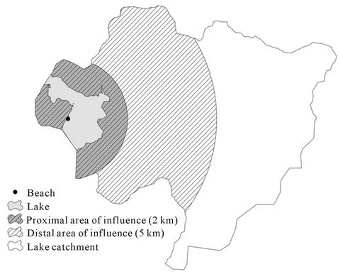
Figure 1. Two buffer zones used to delineate the geographical area influencing the fecal pollution of water bodies in the article of Turgeon et al. (With kind permission from Springer Science +Business Media: Water Quality, Exposure and Health, Fecal Contamination of Recreational Freshwaters: the Effect of Time-Independent Factors, Vol. 3 (2), 2011, 109-118, P. Turgeon et al., Figure 1).
first 2 km.
Although results of these studies differ according to their objectives and methods, one trend seems to emerge. During a dry season, microbiological surface water quality would be more influenced by land use characteristics located nearest the sampling station versus by the whole catchment, reflecting a possible die-off or sedimentation process along watercourses during this period.
5. Quantitatively Measuring These Sources and Factors and Their Association with Fecal Pollution of Recreational Freshwater
After having identified potential sources of fecal contamination and their modulating factors and delineating the area where they should be monitored more closely, the next step should be to quantitatively measure them in the areas of interest. Various sources of data can be used for this such as census data, regional or national thematic maps, and field survey data [14,78-80]. National census data from human populations can be useful for evaluating density or some characteristics such as age or socioeconomic distribution [81]. Census data from animal populations can also provide information on population density and species distribution or contribute to the evaluation of some management practices such as manure spreading [82]. The advantages of this data source are that data are usually standardized at the national level, available freely and for a long period of time. However, census data are collected most of the time by administrative regions or districts or centralized by farms or businesses.
These methods can bring spatial uncertainty which can be very relevant in the context of a hydrological process where the location of the source of contamination in regard to runoff direction and topography can play an important role [83,84]. Moreover, census data are usually constrained in regards to timeline. As an example, in Canada, population census is done every four years and agricultural census every five years, which can prevent availability of up-to-date data [81,82].
Data on landscape, land use, or on some environmental characteristics such as climatic conditions or topography can be acquired from regional or national thematic maps [80,85]. One advantage of using these maps is that one map is usually able to provide data on wide territories for more than one characteristic. Most of the time, data can be relatively easy to extract and thus can be ready to use with little manipulation. Nonetheless, like census processes, thematic maps are usually not performed every year and the timeline can be restrictive in a monitoring context. Furthermore, spatial resolution of these maps may limit their use or contribute to some measurement errors when data are needed for small areas [80]. Field surveys can provide accurate, precise, and up-to-date data on small areas, but one downside of this method is the high cost in terms of time and human and financial resources.
Lastly, land usage and landscape characteristics can also be provided by satellite imagery and more specifically Earth observation imagery [86,87]. These products can provide data on land use and land cover known to influence surface and recreational water quality such as agricultural lands, impervious (built) surfaces, wetlands, and forest areas [88-91]. This source of data has many advantages over more conventional sources. First, satellites can have a very large coverage and thus provide information on wide territories [92,93]. Satellite data from a particular sensor are always collected the same way and usually for a long period of time, allowing for a large amount of repeatable and consistent data which can be very relevant for a monitoring program [94]. Data from Earth observation can be highly precise depending on the sensor; knowing the precise data on characteristics associated with fecal contamination can be very relevant in the context of a hydrological matter. However, some factors can make their use difficult for recreational water monitoring, such as image cost and the expertise and technical resources needed for the gathering, processing, and analysing of those data [95-97]. As all sources of data present advantages and limitations, a combination of more than one source is probably the best way to tackle this step depending on the environment and the recreational waters involved.
Once the environmental characteristics associated with potential sources of fecal contamination and their modulator factors have been measured, it can be pertinent to try to identify which of these determinants have the most influence on recreational waters in the territory of interest. Most of the time, statistical methods that were used to achieve this step were multivariate regression modelling and Pearson’s correlation coefficient [14,77-79,98]. Knowledge resulting from this step could provide the answer to the question: Which beaches have a higher risk of fecal contamination? Identification of those beaches combined with water sampling would provide the basis for an overall evaluation according to the risk and the actual level of fecal pollution, allowing for a better targeted monitoring of recreational waters.
6. Conclusion and Future Directions
Based on a literature review, this paper aimed to suggest and discuss steps that should be followed for the integration of environmental determinants in the monitoring of recreational waters. Initially, potential sources of contamination and factors able to modulate them should be identified. Various sources and factors can be involved and depend on the region of interest. Measuring these sources and factors for monitoring purposes can only be done after delineating the geographical area influencing fecal contamination of recreational waters. No scientific consensus exists on this matter and few studies have participated in the debate. Nevertheless, in dry periods, which largely correspond to the bathing season, the proximal environment seems to play a more important role in the pollution process than the whole catchment does. Studies using mathematical and hydrological modelling would certainly help to bring new knowledge on this topic. Various sources of data can be used to provide information on sources of contamination and modulating factors and could be used to measure them on the geographical area of interest. Since none of them is sufficient in itself to provide all the information needed to fully characterize the proximal environment of recreational waters, a combination of more than one would be the best way to measure environmental characteristics. Some studies have used statistical models to identify the relative importance of environmental characteristics on fecal pollution of recreational waters. Although these models provide relevant information on environmental characteristics associated with a higher risk of fecal contamination and thus can serve as a good working basis for the integration of the monitoring of the environmental determinants of recreational water quality, they do not allow for a full comprehension of the exact processes leading to this pollution. Source attribution methods should be used to better understand these processes and to provide information on a better estimation of the precise contribution of each source of contamination.
Monitoring environmental determinants of water quality should be integrated with monitoring programs of recreational waters. In addition to water testing, it would provide an overall evaluation according to the risk of contamination and the actual level of fecal pollution, promoting in turn good water management actions to ensure safe water quality [13]. Moreover, knowing and monitoring these determinants could promote preventive actions to diminish their impact on water quality. In addition to contributing to better protecting the public, this preventive approach would align with the multi-barrier approach promoted in the domain of water quality [99, 100].
7. Acknowledgements
The author wishes to thank Dr. Pascal Michel of the Public Health Agency of Canada for his helpful comments on this paper.
REFERENCES
- J. B. Rose, P. R. Epstein, E. K. Lipp, B. H. Sherman, S. M. Bernard and J. A. Patz, “Climate Variability and Change in the United States: Potential Impacts on Waterand Foodborne Diseases Caused by Microbiologic Agents [Review],” Environmental Health Perspectives, Vol. 109, Suppl. 2, 2001, pp. 211-221.
- Intergovernmental Panel on Climate Change, “Climate Change 2007: Synthesis Report,” Valencia, Spain, 2007. http://www.ipcc.ch/pdf/assessment-report/ar4/syr/ar4_syr.pdf
- A. Pruss, “Review of Epidemiological Studies on Health Effects from Exposure to Recreational Water,” International Journal of Epidemiology, Vol. 27, No. 1, 1998, pp. 1-9. doi:10.1093/ije/27.1.1
- K. A. Feldman, J. C. Mohle-Boetani, J. Ward, K. Furst, S. L. Abbott, D. V. Ferrero, A. Olsen and S. B. Werner, “A Cluster of Escherichia coli O157: Nonmotile Infections Associated with Recreational Exposure to Lake Water,” Public Health Reports, Vol. 117, No. 4, 2002, pp. 380- 385.
- M. G. Bruce, M. B. Curtis, M. M. Payne, R. K. Gautom, E. C. Thompson, A. L. Bennett and J. M. Kobayashi, “Lake-Associated Outbreak of Escherichia coli O157:H7 in Clark County, Washington, August 1999,” Archives of Pediatrics & Adolescent Medicine, Vol. 157, No. 10, 2003, pp. 1016-1021. doi:10.1001/archpedi.157.10.1016
- A. Wiedenmann, P. Kruger, K. Dietz, J. M. Lopez-Pila, R. Szewzyk and K. Botzenhart, “A Randomized Controlled Trial Assessing Infectious Disease Risks from Bathing in Fresh Recreational Waters in Relation to the Concentration of Escherichia coli, Intestinal Enterococci, Clostridium perfringens and Somatic coliphages,” Environmental Health Perspectives, Vol. 114, No. 2, 2006, pp. 228-236. doi:10.1289/ehp.8115
- B. Sartorius, Y. Andersson, I. Velicko, B. De Jong, M. Löfdahl, K.-O. Hedlund, G. Allestam, C. Wangsell, O. Bergstedt, P. Horal, P. Ulleryd and A. Soderstrom, “Outbreak of Norovirus in Västra Götaland Associated with Recreational Activities at Two Lakes during August 2004,” Scandinavian Journal of Infectious Diseases, Vol. 39, No. 4, 2007, pp. 323-331. doi:10.1080/00365540601053006
- J. M. Fleisher, L. E. Fleming, H. M. Solo-Gabriele, J. K. Kish, C. D. Sinigalliano, L. Plano, S. M. Elmir, J. D. Wang, K. Withum, T. Shibata, M. L. Gidley, A. Abdelzaher, G. Q. He, C. Ortega, X. F. Zhu, M. Wright, J. Hollenbeck and L. C. Backer, “The BEACHES Study: Health Effects and Exposures from Non-Point Source Microbial Contaminants in Subtropical Recreational Marine Waters,” International Journal of Epidemiology, Vol. 39, No. 5, 2010, pp. 1291-1298. doi:10.1093/ije/dyq084
- J. W. Santo Domingo, S. C. Siefring and R. A. Haugland, “Real-Time PCR Method to Detect Enterococcus faecalis in Water,” Biotechnology Letters, Vol. 25, No. 3, 2003, pp. 261-265. doi:10.1023/A:1022303118122
- T. J. Wade, R. L. Calderon, E. Sams, M. Beach, K. P. Brenner, A. H. Williams and A. P. Dufour, “Rapidly Measured Indicators of Recreational Water Quality Are Predictive of Swimming-Associated Gastrointestional Illness,” Environmental Health Perspectives, Vol. 114, No. 1, 2006, pp. 24-28. doi:10.1289/ehp.8273
- G. A. Olyphant and R. L. Whitman, “Elements of a Predictive Model for Determining Beach Closures on a Real Time Basis: The Case of 63rd Street Beach Chicago,” Environmental Monitoring & Assessment, Vol. 98, No. 1-3, 2004, pp. 175-190. doi:10.1023/B:EMAS.0000038185.79137.b9
- D. S. Francy, R. A. Darner and E. E. Bertke, “Models for Predicting Recreational Water Quality at Lake Erie Beaches,” US Geological Survey. Scientific Investigations Report 2006-5192, 2006.
- World Health Organization, “Guidelines for Safe Recreationnal Water Environments. Coastal and Fresh Waters,” Geneva, Switzerland, 2003, http://www.who.int/water_sanitation_health/bathing/srwe1/en/
- P. Turgeon, P. Michel, P. Levallois, M. Archambault and A. Ravel, “Fecal Contamination of Recreational Freshwaters: The Effect of Time-Independent Agroenvironmental Factors,” Water Quality, Exposure and Health, Vol. 3, No. 2, 2011, pp. 109-118. doi:10.1007/s12403-011-0048-5
- M. L. Hutchison, L. D. Walters, S. M. Avery, B. A. Synge and A. Moore, “Levels of Zoonotic Agents in British Livestock Manures,” Letters in Applied Microbiology, Vol. 39, No. 2, 2004, pp. 207-214. doi:10.1111/j.1472-765X.2004.01564.x
- E. M. Moriarty, L. W. Sinton, M. L. Mackenzie, N. Karki and D. R. Wood, “A Survey of Enteric Bacteria and Protozoans in Fresh Bovine Faeces on New Zealand Dairy Farms,” Journal of Applied Microbiology, Vol. 105, No. 6, 2008, pp. 2015-2025. doi:10.1111/j.1365-2672.2008.03939.x
- R. Calderon, M. E. and A. Dufour, “Health Effects of Swimmers and Non-Point Sources of Contaminated Water,” International Journal of Environmental Health Research, Vol. 1, 1991, pp. 21-31.
- J. M. Colford Jr., T. J. Wade, K. C. Schiff, C. C. Wright and J. F. Griffith, “Water Quality Indicators and the Risk of Illness at Beaches with Non-Point Sources of Fecal Contamination,” Epidemiology, Vol. 18, 2007, pp. 27-35. doi:10.1097/01.ede.0000249425.32990.b9
- V. P. Olivieri, K. Kawata and S. H. Lim, “Microbiological Impacts of Storm Sewer Overflows: Some Aspects of the Implication of Microbiological Indicators for Receiving Waters,” In: J. B. Ellis, Ed., Urban Discharges and Receiving Water Quality Impacts, Pergamon Press, Oxford, 1989, pp. 47-54.
- Environment Canada, “Wastewater Management,” Environment Canada, 2009. http://www.ec.gc.ca/eu-ww/default.asp?lang=En&n=0FB32EFD-1
- United States Environmental Protection Agency, “Report to Congress. Impacts and Control of CSOs and SSOs,” Washington DC, 2004. http://cfpub.epa.gov/npdes/cso/cpolicy_report2004.cfm
- J. A. Castro-Hermida, I. Garcia-Presedo, A. Almeida, M. Gonzalez-Warleta, J. M. C. Da Costa and M. Mezo, “Contribution of Treated Wastewater to the Contamination of Recreational River Areas with Cryptosporidium spp. and Giardia duodenalis,” Water Research, Vol. 42, No. 13, 2008, pp. 3528-3538. doi:10.1016/j.watres.2008.05.001
- J. Marsalek and Q. Rochfort, “Urban Wet-Weather Flows: Sources of Fecal Contamination Impacting on Recreational Waters and Threatening Drinking-Water Sources,” Journal of Toxicology and Environmental Health, Vol. 67, No. 20-22, 2004, pp. 1765-7717. doi:10.1080/15287390490492430
- P. Payment, R. Plante and P. Cejka, “Removal of Indicator Bacteria, Human Enteric Viruses, Giardia Cysts, and Cryptosporidium Oocysts at a Large Wastewater Primary Treatment Facility,” Canadian Journal of Microbiology, Vol. 47, No. 3, 2001, pp. 188-193.
- C. P. Gerba, “Assessment of Enteric Pathogen Shedding by Bathers during Recreational Activity and its Impact on Water Quality,” Quantitative Microbiology, Vol. 2, 2000, pp. 55-68.
- D. Sunderland, T. K. Graczyk, L. Tamang and P. N. Breysse, “Impact of Bathers on Levels of Cryptosporidium parvum Oocysts and Giardia lamblia Cysts in Recreational Beach Waters,” Water Research, Vol. 41, No. 15, 2007, pp. 3483-3489. doi:10.1016/j.watres.2007.05.009
- J. Blostein, “Shigellosis from Swimming in a Park Pond in Michigan,” Public Health Reports, Vol. 106, No. 3, 1991, pp. 317-322.
- W. E. Keene, J. M. McAnulty, F. C. Hoesly, L. P. Williams, K. Hedberg, G. L. Oxman, T. J. Barrett, M. A. Pfaller and D. W. Fleming, “A Swimming-Associated Outbreak of Hemorrhagic Colitis Caused by Escherichia coli O157:H7 and Shigella Sonnei,” New England Journal of Medicine, Vol. 331, No. 9, 1994, pp. 579-584. doi:10.1056/NEJM199409013310904
- M. Iwamoto, G. Hlady, M. Jeter, C. Burnett, C. Drenzek, S. Lance, J. Benson, D. Page and P. Blake, “Shigellosis among Swimmers in a Freshwater Lake,” Southern Medical Journal, Vol. 98, No. 8, 2005, pp. 774-778. doi:10.1097/01.smj.0000172764.14147.e5
- T. K. Graczyk, D. Sunderland, G. N. Awantang, Y. Mashinski, F. E. Lucy, Z. Graczyk, L. Chomicz and P. N. Breysse, “Relationships among Bather Density, Levels of Human Waterborne Pathogens, and Fecal Coliform Counts in Marine Recreational Beach Water,” Journal of Parasitology Research, Vol. 106, No. 5, 2010, pp. 1103- 1108. doi:10.1007/s00436-010-1769-2
- S. Hill, J. M. Cheney, G. F. Taton-Allen, J. S. Reif, C. Bruns and M. R. Lappin, “Prevalence of Enteric Zoonotic Organisms in Cats,” Journal of the American Vetrinary Medical Association, Vol. 216, No. 5, 2000, pp. 687-692. doi:10.2460/javma.2000.216.687
- T. Hackett and M. R. Lappin, “Prevalence of Enteric Pathogens in Dogs of North-Central Colorado,” Journal of the American Animal Hospital Association, Vol. 39, 2003, pp. 52-56.
- L. R. Fogarty, S. K. Haack, M. J. Wolcott and R. L. Whitman, “Abundance and Characteristics of the Recreational Water Quality Indicator Bacteria Escherichia coli and Enterococci in Gull Faeces,” Journal of Applied Microbiology, Vol. 94, No. 5, 2003, pp. 865-878. doi:10.1046/j.1365-2672.2003.01910.x
- S. K. Haack, L. R. Fogarty and C. Wright, “Escherichia coli and Enterococci at Beaches in the Grand Traverse Bay, Lake Michigan: Sources, Characteristics, and Environmental Pathways,” Environmental Science & Technology, Vol. 37, No. 15, 2003, pp. 3275-3282. doi:10.1021/es021062n
- Z. Hubalek, “An Annotated Checklist of Pathogenic Microorganisms Associated with Migratory Birds [Review],” Journal of Wildlife Diseases, Vol. 40, No. 4, 2004, pp. 639-659.
- K. J. Meyer, C. M. Appletoft, A. K. Schwemm, K. Uzoigwe and E. J. Brown, “Determining the Source of Fecal Contamination in Recreational Waters,” Journal of Environmental Health, Vol. 68, No. 1, 2005, pp. 25-30.
- T. A. Edge and S. Hill, “Multiple Lines of Evidence to Identify the Sources of Fecal Pollution at a Freshwater Beach in Hamilton Harbour, Lake Ontario,” Water Research, Vol. 41, No. 16, 2007, pp. 3585-3594. doi:10.1016/j.watres.2007.05.012
- T. K. Graczyk, A. C. Majewska and K. J. Schwab, “The Role of Birds in Dissemination of Human Waterborne Enteropathogens,” Trends in Parasitology, Vol. 24, No. 2, 2008, pp. 55-59. doi:10.1016/j.pt.2007.10.007
- V. R. Simpson, “Wild Animals as Reservoirs of Infectious Diseases in the UK,” The Veterinary Journal, Vol. 163, No. 2, 2002, pp. 128-146. doi:10.1053/tvjl.2001.0662
- K. Handeland, L. L. Nesse, A. Lillehaug, T. Voikoren, B. Djonne and B. Bergsjo, “Natural and Experimental Salmonella typhimurium Infections in Foxes (Vulpes vulpes),” Veterinary Microbiology, Vol. 132, No. 1-2, 2008, pp. 129-134. doi:10.1016/j.vetmic.2008.05.002
- C. Jardine, R. J. Reid-Smith, N. Janecko, M. Allan and S. A. McEwen, “Salmonella in Racoons (Proycon lotor) in Southern Ontario, Canada,” Journal of Wildlife Diseases, Vol. 47, No. 2, 2011, pp. 344-351.
- R. Majdoub, C. Côté, M. Labadi, K. Guay and M. Généreux, “Impact de l’Utilisation des Engrais de Ferme sur la Qualité Microbiologique de l’eau Souterraine,” Instituts de Recherche et de Développement en AgroEnvironnement, Québec, 2003.
- P. Chevalier, P. Levallois and P. Michel, “Infections Entériques d’Origine Hydrique Potentiellement Associées à la Production Animale: Revue de la Littérature,” Vecteur Environnement, Vol. 37, No. 2, 2004, pp. 90-106.
- Government of Canada, “Waterborne Outbreak of Gastroenteritis Associated with a Contaminated Municipal Water Supply, Walkerton, Ontario, May-June 2000,” Canada Communicable Disease Report, Vol. 26, No. 20, 2000, pp. 170-173.
- J. A. Thurston-Enriquez, J. E. Gilley and B. Eghball, “Microbial Quality of Runoff Following Land Application of Cattle Manure and Swine Slurry,” Journal of Water & Health, Vol. 3, No. 2, 2005, pp. 157-171.
- M. C. Ramos, J. N. Quinton and S. F. Tyrrel, “Effects of Cattle Manure on Erosion Rates and Runoff Water Pollution by Faecal Coliforms,” Journal of Environmental Management, Vol. 78, No. 1, 2006, pp. 97-101. doi:10.1016/j.jenvman.2005.04.010
- Health Canada, “Guidelines for Canadian Recreationnal Water Quality,” Ottawa, 1992. http://www.hc-sc.gc.ca/ewh-semt/pubs/water-eau/guide_water-1992-guide_eau/index-eng.php
- X. P. Jiang, J. Morgan and M. P. Doyle, “Fate of Escherichia coli O157:H7 during Composting of Bovine Manure in a Laboratory-Scale Bioreactor,” Journal of Food Protection, Vol. 66, No. 1, 2003, pp. 25-30.
- L. M. Avery, K. Killham and D. L. Jones, “Survival of E. coli O157:H7 in Organic Wastes Destined for Land Application,” Journal of Applied Microbiology, Vol. 98, No. 4, 2005, pp. 814-22. doi:10.1111/j.1365-2672.2004.02524.x
- A. J. A. Vinten, J. T. Douglas, D. R. Lewis, M. N. Aitken and D. R. Fenlon, “Relative Risk of Surface Water Pollution by E. coli Derived from Faeces of Grazing Animals Compared to Slurry Application,” Soil Use & Management, Vol. 20, No. 1, 2004, pp. 13-22. doi:10.1079/SUM2004214
- S. M. Avery, A. Moore and M. L. Hutchison, “Fate of Escherichia coli Originating from Livestock Faeces Deposited Directly onto Pasture,” Letters in Applied Microbiology, Vol. 38, No. 5, 2004, pp. 355-359. doi:10.1111/j.1472-765X.2004.01501.x
- L. W. Sinton, R. R. Braithwaite, C. H. Hall and M. L. Mackenzie, “Survival of Indicator and Pathogenic Bacteria in Bovine Feces on Pasture,” Applied & Environmental Microbiology, Vol. 73, No. 24, 2007, pp. 7917- 7925. doi:10.1128/AEM.01620-07
- R. K. Hubbard, G. L. Newton and G. M. Hill, “Water Quality and the Grazing Animals,” Journal of animal science, Vol. 82, 2004, pp. E255-E263.
- P. Rodgers, C. Soulsby, C. Hunter and J. Petry, “Spatial and Temporal Bacterial Quality of a Lowland Agricultural Stream in Northeast Scotland,” The Science of the total Environment, Vol. 314-316, 2003, pp. 289-302. doi:10.1016/S0048-9697(03)00061-5
- J. A. Entry, R. K. Hubbard, J. E. Thies and J. J. Fuhrmann, “The Influence of Vegetation in Riparian Filterstrips on Coliform Bacteria: I. Movement and Survival in Water,” Journal of Environmental Quality, Vol. 29, No. 4, 2000, pp. 1206-1214. doi:10.2134/jeq2000.00472425002900040026x
- R. M. Roodsari, D. R. Shelton, A. Shirmohammadi, Y. A. Pachepsky, A. M. Sadeghi and J. L. Starr, “Fecal Coliform Transport as Affected by Surface Condition,” Transactions of the ASAE, Vol. 48, No. 3, 2005, pp. 1055-1061.
- T. J. Sullivan, J. A. Moore, D. R. Thomas, E. Mallery, K. U. Snyder, M. Wustenberg, J. Wustenberg, S. D. Mackey and D. L. Moore, “Efficacy of Vegetated Buffers in Preventing Transport of Fecal Coliform Bacteria from Pasturelands,” Environmental Management, Vol. 40, No. 6, 2007, pp. 958-965. doi:10.1007/s00267-007-9012-3
- É. Gagnon and G. Gangbazo, “Efficacité des Bandes Riveraines: Analyse de la Documentation Scientifique et Perspectives,” Ministère du Développment Durable, de l’Environnement et des Parcs du Québec, Québec, 2007.
- C. Kao and M. Wu, “Control of Non-Point Source Pollution by a Natural Wetlands,” Water Science and Technology, Vol. 43, No. 5, 2001, pp. 169-174.
- [61] A. K. Knox, A. R. Dahlgren, K. W. Tate and E. R. Atwill, “Efficacy of Natural Wetlands to Retain Nutrient, Sediment and Microbial Polluants,” Journal of Environmental Quality, Vol. 37, 2008, pp. 1837-1846. doi:10.2134/jeq2007.0067
- [62] M. Matteo, T. Randhir and D. Bloniarz, “WatershedScale Impacts of Forest Buffers on Water Quality and Runoff in Urbanizing Environment,” Journal of Water Resources Planning and Management, Vol. 132, No. 3, 2006, pp. 144-152. doi:10.1061/(ASCE)0733-9496(2006)132:3(144)
- [63] J. Abu-Ashour and H. Lee, “Transport of Bacteria on Sloping Soil Surfaces by Runoff,” Environmental Toxicology, Vol. 15, No. 2, 2000, pp. 149-153. doi:10.1002/(SICI)1522-7278(2000)15:2<149::AID-TOX11>3.0.CO;2-O
- [64] C. Ferguson, A. M. D. Husman, N. Altavilla, D. Deere and N. Ashbolt, “Fate and Transport of Surface Water Pathogens in Watersheds [Review],” Critical Reviews in Environmental Science & Technology, Vol. 33, No. 3, 2003, pp. 299-361. doi:10.1080/10643380390814497
- [65] I. D. Ogden, D. R. Fenlon, A. J. A. Vinten and D. Lewis, “The fate of Escherichia coli O157 in Soil and Its Potential to Contaminate Drinking Water,” International Journal of Food Microbiology, Vol. 66, No. 1-2, 2001, pp. 111-117. doi:10.1016/S0168-1605(00)00508-0
- [66] D. Trevisan, J. Y. Vansteelant and J. M. Dorioz, “Survival and Leaching of Fecal Bacteria after Slurry Spreading on Mountain Hay Meadows: Consequences for the Management of Water Contamination Risk,” Water Research, Vol. 36, No. 1, 2002, pp. 275-283. doi:10.1016/S0043-1354(01)00184-1
- [67] R. W. Muirhead, R. P. Collins and P. J. Bremer, “Interaction of Escherichia coli and Soil Particles in Runoff,” Applied and Environmental Microbiology, Vol. 72, No. 5, 2006, pp. 3406-3411. doi:10.1128/AEM.72.5.3406-3411.2006
- [68] F. C. Curriero, J. A. Patz, J. B. Rose and S. Lele, “The Association between Extreme Precipitation and Waterborne Disease Outbreaks in the United States, 1948- 1994,” American Journal of Public Health, Vol. 91, No. 8, 2001, pp. 1194-1199. doi:10.2105/AJPH.91.8.1194
- [69] D. F. Charron, M. K. Thomas, D. Waltner-Toews, J. J. Aramini, T. Edge, R. A. Kent, A. R. Maarouf and J. Wilson, “Vulnerability of Waterborne Diseases to Climate Change in Canada: A Review,” Journal of Toxicology & Environmental Health Part A, Vol. 67, No. 20-22, 2004, pp. 1667-1677. doi:10.1080/15287390490492313
- [70] J. A. Patz, S. J. Vavrus, C. K. Uejio and S. L. McLellan, “Climate Change and Waterborne Disease Risk in the Great Lakes Region of the US,” American Journal of Preventive Medicine, Vol. 35, No. 5, 2008, pp. 451-458. doi:10.1016/j.amepre.2008.08.026
- [71] R. L. Whitman, M. B. Nevers, G. C. Korinek and M. N. Byappanahalli, “Solar and Temporal Effects on Escherichia coli Concentration at a Lake Michigan Swimming Beach,” Applied and Environmental Microbiology, Vol. 70, No. 7, 2004, pp. 4276-4285. doi:10.1128/AEM.70.7.4276-4285.2004
- [72] S. R. Crane and J. A. Moore, “Modeling Enteric Bacterial Die-Off: A Review,” Water Air soil Pollution, Vol. 27, 1986, p. 411. doi:10.1007/BF00649422
- [73] J. Abu-Ashour, D. M. Joy, H. Lee, H. R. Whiteley and S. Zelin, “Transport of Microorganisms through Soil,” Water, Air, & Soil Pollution, Vol. 75, 1994, pp. 141-158. doi:10.1007/BF01100406
- [74] R. C. Jamieson, R. J. Gordon, K. E. Sharples, G. W. Stratton and A. Madani, “Movement and Persistence of Fecal Bacteria in Agricultural Soils and Subsurface Drainage Water: A Review,” Canadian Biosystems Engineering, Vol. 44, No. 1, 2002, pp. 1-9.
- [75] M. M. Lau, S. C. Ingham and A. R. Arment, “Survival of Faecal Indicator Bacteria in Bovine Manure Incorporated into Soil,” Letters in Applied Microbiology, Vol. 33, 2001, p. 131.
- [76] L. Johnson and S. Gage, “Landscape Approaches to the Analysis of Aquatic Ecosystems,” Freshwater Biology, Vol. 37, No. 1, 1997, pp. 113-132. doi:10.1046/j.1365-2427.1997.00156.x
- [77] L. Sliva and D. D. Williams, “BUFFER zone versus Whole Catchment Approaches to Studying Land Use Impact on River Water Quality,” Water Research, Vol. 35, No. 14, 2001, pp. 3462-3472. doi:10.1016/S0043-1354(01)00062-8
- [78] J. Crowther, M. D. Wyer, M. Bradford, D. Kay, C. A. Francis and W. G. Knisel, “Modelling Faecal Indicator Concentrations in Large Rural Catchments Using Land Use and Topographic Data,” Journal of Applied Microbiology, Vol. 94, No. 6, 2003, pp. 962-973. doi:10.1046/j.1365-2672.2003.01877.x
- [79] J. Crowther, D. Kay and M. D. Wyer, “Faecal-Indicator Concentrations in Waters Draining Lowland Pastoral Catchments in the UK: Relationships with Land Use and Farming Practices,” Water Research, Vol. 36, No. 7, 2002, pp. 1725-1734. doi:10.1016/S0043-1354(01)00394-3
- [80] D. Kay, M. Wyer, J. Crowther, C. Stapleton, M. Bradford, A. McDonald, J. Greaves, C. Francis and J. Watkins, “Predicting Faecal Indicator Fluxes Using Digital Land Use Data in the UK’s Sentinel Water Framework Directive Catchment: The Ribble Study,” Water Research, Vol. 39, No. 16, 2005, pp. 3967-3981. doi:10.1016/j.watres.2005.07.006
- [81] D. Kay, S. Anthony, J. Crowther, B. J. Chambers, F. A. Nicholson, D. Chadwick, C. M. Stapleton and M. D. Wyer, “Microbial Water Pollution: A Screening Tool for Initial Catchment-Scale Assessment and Source Apportionment,” Science of the Total Environment, Vol. 408, No. 23, 2010, pp. 5646-5656. doi:10.1016/j.scitotenv.2009.07.033
- [82] Statistics Canada, “2006 Census,” Statistics Canada, 2007. http://www12.statcan.gc.ca/census-recensement/index-eng.cfm
- [83] Statistics Canada, “2006 Agriculture Census,” Statistics Canada, 2008. http://www.statcan.gc.ca/ca-ra2006/index-eng.htm
- [84] P. D’Arcy and R. Carignan, “Influence of Catchment Topography on Water Chemistry in Southeastern Quebec Shield Lakes,” Canadian Journal of Fisheries & Aquatic Sciences, Vol. 54, 1997, pp. 2215-2227.
- [85] P. Turgeon, P. Michel, P. Levallois, P. Chevalier, D. Daignault, B. Crago, R. Irwin, S. A. McEwen, N. F. Neumann and M. Louie, “Agroenvironmental Determinants Associated with the Presence of AntimicrobialResistant Escherichia coli in Beach Waters in Quebec, Canada,” Zoonoses and Public Health, Vol. 58, No. 6, 2011, pp. 432-439.
- [86] D. W. McKenney, M. F. Hutchinson, J. L. Kesteven and L. A. Venier, “Canada’s Plant Hardiness Zones Revisited Using Modern Climate Interpolation Techniques,” Canadian Journal of Plant Sciences, Vol. 81, 2001, pp. 129- 143.
- [87] J. D. Boone, K. C. McGwire, E. W. Otteson, R. S. DeBaca, E. A. Kuhn, P. Villard, P. F. Brussard and S. C. St Jeor, “Remote Sensing and Geographic Information Systems: Charting Sin Nombre Virus Infections in Deer Mice,” Emerging Infectious Diseases, Vol. 6, No. 3, 2000, pp. 248-258.
- [88] A. Leblond, A. Sandoz, G. Lefebvre, H. Zeller and D. J. Bicout, “Remote Sensing Based Identification of Environmental Risk Factors Associated with West Nile Disease in Horses in Camargue, France,” Preventive Veterinary Medicine, Vol. 79, No. 1, 2007, pp. 20-31.
- [89] L. R. Beck, B. M. Lobitz and B. L. Wood, “Remote Sensing and Human Health: New Sensors and New Opportunities,” Emerging Infectious Diseases, Vol. 6, No. 3, 2000, pp. 217-227.
- [90] S. Kalluri, P. Gilruth, D. Rogers and M. Szczur, “Surveillance of Arthropod Vector-Borne Infectious Diseases Using Remote Sensing Techniques: A Review Art. No. e116 [Review],” PLoS Pathogens, Vol. 3, No. 10, 2007, pp. 1361-1371.
- [91] J. B. Campbell, “Introduction to Remote Sensing,” The Guilford Press, New York, 2007.
- [92] Y. Zhang, B. Guindon, K. Sun and L. Sun, “Remote Sensing for Improving Understanding on Canadian Urbanization,” Canada Centre for Remote Sensing, Natural Resources Canada, 2010. http://www.ccrs.nrcan.gc.ca/optical/curlus_e.php
- [93] J. P. Messina and K. A. Crews-Meyer, “A Historical Perspective on the Development of Remotely Sensed Data as Applied to Medical Geography,” In: D. P. Albert, W. M. Geslier and B. Levrgood, Eds., Spatial Analysis, GIS, and Remote Sensing Applications in the Health Sciences, Ann Arbor Press, Chelsea, 2000, pp. 129-146.
- [94] United Nations Office for Outer Space Affairs, “Space Solutions for the World’s Problems,” Vienna, 2005. http://www.oosa.unvienna.org/pdf/publications/IAM2005E.pdf
- [95] S. J. Goetz, S. D. Prince and J. Small, “Advances in Satellite Remote Sensing of Environmental Variables for Epidemiological Applications,” In: S. I. Hay, S. E. Randolph and D. J. Rogers, Eds., Remote Sensing and Geographical Information Systems in Epidemiology, Elsevier Sciences, Oxford, 2002, pp. 289-309.
- [96] V. R. M. Correia, M. S. Carvalho, P. C. Sabroza and C. H. Vacsoncelos, “Remote Sensing as a Tool to Survey Endemic Diseases in Brazil,” Cad. Saûde Pûblica, Vol. 20, No. 4, 2004, pp. 891-904.
- [97] B. C. Rundquist, C. J. Henrie and E. J. Grewe, “Internet Acess to Remotely Sensed Data: Satellite Imaging Made Commonplace,” Journal of Map & geography Libraries, Vol. 2, No. 2, 2006, pp. 21-30.
- [98] S. N. V. Kalluri and T. J. Schmugge, “Application of Remote Sensing in Agriculture and Soil Science,” In: K. R. Krishna, Ed., Soil Fertility and Crop Production, Chapter 18, Science Publisher, Enfield, 2002, 465 p.
- [99] D. Hampson, J. Crowther, I. Bateman, D. Kay, P. Posen, C. Stapleton, M. Wyer, C. Fezzi, P. Jones and J. Tzanopoulos, “Predicting Microbial Pollution Concentrations in UK Rivers in Response to Land Use Change,” Water Research, Vol. 44, No. 16, 2010, pp. 4748-4759.
- [100] Canadian Federal-Provincial-Territorial Committee on Environmental and Occupational Health and the Canadian Council of Ministers of the Environment, “From Source to Tap: The Multi-Barrier Approach to Safe Drinking Water,” 2002. http://www.hc-sc.gc.ca/ewh-semt/alt_formats/hecs-sesc/pdf/water-eau/tap-source-robinet/tap-source-robinet-eng.pdf
- [101] Ministry for the Environment, New Zealand, “Draft Users’ Guide: National Environmental Standard for Sources of Human Drinking Water,” 2012 http://www.mfe.govt.nz/publications/rma/nes-draft-sources-human-drinking-water/html/index.html