Journal of Environmental Protection
Vol. 3 No. 9 (2012) , Article ID: 22643 , 12 pages DOI:10.4236/jep.2012.39114
An Investigation of the Carbon Neutrality of Wood Bioenergy
![]()
1The “Forest and Economics Program” at Resources for the Future, Washington DC, USA; 2Ohio State University, Columbus, USA.
Email: Sedjo@rff.org
Received May 12th, 2012; revised June 14th, 2012; accepted July 15th, 2012
Keywords: Carbon; Carbon Footprint; Carbon Neutrality; Bioenergy; Forest; Harvests; Anticipation; Rational Expectations
ABSTRACT
Wood biomass has been viewed as “carbon neutral”—its uses as energy have a zero carbon footprint. Some observers argue that the use of wood biofuels will result in a decrease of the forest stock and a net reduction of the carbon captured in the forest. Such assessments take a static, accounting view of forest systems and do not consider the effects of management in renewing the forest and increasing its extent or ability to sequester carbon. This paper addresses the carbon neutrality debate using a dynamic optimization forest management model to examine the effect on the existing and future forests of a changing demand for wood biomass. The results show that under market optimizing conditions, when future demand is anticipated to increase for significant periods, the response of managers will be to increase the intensity of forest production thereby offsetting much of the carbon released in bioenergy production.
1. Introduction
Until recently, the conventional wisdom was that the use of wood energy as a substitute for fossil fuels would reduce net carbon emissions, since the wood biomass would substitute for fossil fuels and wood, being a renewable resource, would recapture the emitted carbon as the forest regrows. Essentially, the carbon emitted by biomass energy would be recycled back into the forest with the assumption being that the forest stock would remain unchanged [1]. A new argument is that the use of wood biofuels will decrease the forest stock and thus reduce the net carbon captured in the forest. This would offset some or all of the gains from the decrease in fossil fuel use [2-5].
The argument involves intertemporal issues related to the direct use of wood for biomass energy. Wood from the forest can be used as a feedstock for biofuels (e.g., ethanol) or directly combusted to provide energy for electrical power generation. Although the long-term net change in the amount of carbon captured in the forest may be zero, the new argument runs, in the shorter term the initial large emissions will not be fully offset by regrowth, and so using wood biomass energy will generate substantial near-term increases in atmospheric carbon. Additionally, Seachinger et al. [6,7] and Fargione et al. [8] argue that land-use changes might be associated with the greater use of biofuels. For example, high grain prices may cause forestland clearing for cropping, thereby reducing the overall forest and the total carbon stock in that forest.
Most such assessments of the relationship between the carbon sequestered in the forest and net carbon emissions associated with wood bioenergy take an accounting view of a static forest stand. Even when making an assessment over time each stand and each period is treated more or less independently of other stands and periods. For example, in studying the carbon neutrality issue in wood biomass production, the Manomet report’s authors analyzed an individual mature forest stand and independent exogenous harvest decisions.
In fact, however, forestry is a dynamic system in which markets generate changes in management on a broad scale involving multiple stands and multiple forests. Changes in demand in one forest or one stand will be transmitted throughout the multiforest system. A decision to harvest in one forest in a particular time period involves related forest management decisions for other stands, other forests, and other time periods. If they expect future demand to increase, forest managers behave differently than if they expect it to be constant or lower. Higher expected future prices encourage forest expansion, with more active forestland management, tree planting, and silviculture. Indeed, if near-term price trends are expected to rise, current harvest can actually decline as managers “conserve” the wood for future sale in a higher-price period. This phenomenon is not limited to the behavior of one forest manager on one forest but rather will be transmitted via market signals (prices) throughout the system to all forest managers. In a world of scarce energy with rising prices, where biomass is beginning to play a substantive role, future wood prices can be expected to rise. Indeed, some industrial wood mills anticipate having to compete with the biomass feedstock market, and concerns about rising wood prices may well be valid [9].
This paper uses a well-known dynamic optimization forest management model to examine the effect of changing wood biomass demand on the existing forest and the amount of carbon captured by the forest system. We examine how the intertemporal path of forest carbon stocks will change if the increased use of wood for bioenergy increases the draw on forest stocks. The approach uses a general stylized forest sector model to examine the effects of an increase in the use of wood biomass energy on the amount of carbon captured in the forest over time under several hypothetical conditions. In the dynamic forest management model, management activities over time respond to current and anticipated market conditions that maximize financial returns to the forest, under alternative scenarios with different rates of demand growth, elasticities of forestland supply, and growth-and-yield functions. We focus on situations where the market for biomass energy is expected to increase substantially, primarily over a 40-year period, although we also look at situations of declining biomass energy demand.
2. The Role of Rational Expectations in Forest Management
Muth [10] noted that earlier intertemporal analysis ignored expectations of future in the management decisions, instead basing behavioral assumptions on past experience, even though future expectations are often far different from past experience. This is certainly the case for biomass energy, since no past experience exists with biomass becoming a major substitute for fossil fuels. Takayama and Judge [11] developed forward-looking spatial and temporal price and allocation models that built future expectations explicitly into prior management decisions. These “rational expectations” models are now commonly used in forestry projections, including the Timber Supply Model [12,13] and the Forest and Agricultural Sector Optimization Model (FASOM) model [14-16]. Although individual expectations may turn out to be incorrect, the approach assumes only that individual decisions are correct on average. This approach contrasts with earlier modeling techniques in forestry, in which current-period decisions were based entirely on current and past conditions: future expectations were not allowed to directly inform current decisions [17].
Note that decisions based on anticipated future conditions are not unusual in management. The common application of a benefit-cost analysis, for example, compares current investment costs with the value of future benefits. Obviously, future benefits are only anticipated and not known with certainty. Judgments are made about likely future economic conditions and market prices, and the cost of the investment is compared with anticipated future conditions to determine the investment’s economic viability.
3. Analytical Methods
We use a dynamic programming model to examine the relationship between carbon in a forest and the use of forest biomass for energy production. The approach begins with a simple dynamic forest model of a multiage, regulated, sustainable forest capable of continuously producing a consistent harvested product. This hypothetical stylized forest model is used to examine the implications of changes in demand on forest carbon under different conditions—how the use of wood for biomass energy affects the volume of carbon in the forest stock and under what conditions might that stock decline, remain constant, or increase.
Our model addresses a dynamic forest system rather than a single static stand. The dynamic optimization approach solves the entire multiple-stand intertemporal system simultaneously, with the future conditions and prices directly affecting current decisions. The biomass price is determined endogenously in a way that maximizes the present value of the net surplus of the wood biomass market and thereby reflects the scarcity of timber stocks. Such a perspective changes the forest dynamic. Trees are planted in anticipation of their future use as biofuel, and the carbon released upon the burning of the wood was previously sequestered in the earlier (anticipating) biological growth process. From a broad forest system perspective, biomass burning releases not new carbon but carbon that was previously sequestered in anticipation of future biomass burning.
Forestry, by its nature, involves many intertemporal decisions that take place over decades. Typically, tree planting involves current costs and intervening management costs in anticipation of benefits (returns) that are commonly delayed for at least two decades and often much longer. Figure 1, for example, shows that tree planting in the United States rose after 1950 in anticipation of future wood shortages as the nation was expected to gradually draw down old-growth stocks of timber in the face of rising demand. The graph indicates that over a 50-year period, about 40 million acres of forest was planted, most of it by the private sector for commercial purposes. Today, most US harvests come from planted or
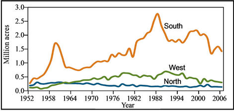
Figure 1. Forest planting in the United States by region, 1952- 2006. Source: US forest resource facts and historical trends, 2009, http://fia.fs.fed.us/library/brochures/default.asp.
second-growth forests. Thus, it ought not to be surprising that the expectation of future biomass energy markets would encourage the creation of biomass stocks in anticipation.
4. The Model
A continuous time optimal control model is presented below. The basic model is a simple variant of a model used in the literature and discussed above. The objective of this model posits that a social planner attempts to maximize the net present value of net surplus in wood biomass markets. Net surplus is defined as the area between the biomass demand curve and the land rent cost. Modifying Sohngen and Sedjo [18] the social planner’s problem is thus:
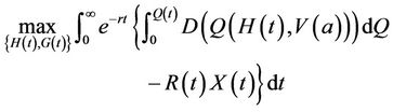 (1)
(1)
s.t
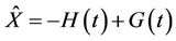 (2)
(2)
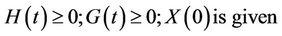 D(∙) is a downwardsloping demand function given the wood biomass quantity per period. Q(∙) is the total quantity harvested generated by the demand function. H(∙) is the hectares harvested, G(∙) the forest area, and V(a) is the wood biomass yield function, where a is the age of trees harvested. R(∙) represents land rent or the opportunity cost of maintaining land as forest rather than converting it for alternative uses. X(∙) is forestland hectares. r is the interest rate, which should reflect the risks associated with carbon uptake service (e.g., fire risk, slower-than-expected tree growth). The state variable here is X(t). The choice variables are H(t) and G(t). The state variable will vary over time according to Equation (2), where
  is the increased hectares of forest between the current period and the next period.
We further modify the earlier model in which forestland area is fixed, to allow the area of wood biomass to expand or decrease by plantation and harvest (Equation (2)). Some harvested land may not be replanted, thereby falling out of forest, and additional land may be converted to forest. These adjustments need not release significant amounts of carbon above that captured by demand. Although only one growth function is used in this paper, analysis with other reasonable growth functions provides the same general results. Finally, although silvicultural practices can increase the wood (and carbon) volume over short periods (e.g., through tree improvement or fertilization), the only management practices allowed in this analysis are adjusting the amount of land in forest and the length of the timber rotation in the context of a regulated forest. Thus, the results tend to be conservative.
The approach is to use a general stylized forest sector model to examine the effects of an increase in the use of wood biomass energy on the amount of carbon captured in the forest over time under several hypothetical conditions. These effects will be examined for different rates of demand growth and different elasticities of forestland supply. Also, the relation of the initial increase in demand to equilibrium conditions is examined.
The model parameters and values for the representative forest are given in Table 1. As noted, the model assumes a regulated forest—that is, an even-aged forest where harvest acres are replanted in the next time period and management is driven by profit-maximizing economic considerations. In the scenarios, described in Table 2, we vary the underlying conditions—level of demand change, land supply elasticity, timber yield function—to assess how the amount of forest carbon might change.
The initial conditions provide for a regulated forest with a given amount of forestland. In all scenarios but the Base Case, the forests are initially in equilibrium under the baseline demand condition where price reflects current demand for wood biomass for energy with the wood volume forthcoming as the harvest. The forest is homogeneous with a stand growth-and-yield function applied to each ha. The amount of carbon captured is a fixed percentage of the forest volumes, as indicated above. To simplify the analysis, we assume that all the harvested wood is used as feedstock for bioenergy and the carbon in the wood harvested is immediately released into the atmosphere. To avoid dealing with a separate type of problem, the amount of waste wood is assumed to be zero. However, these assumptions are not necessary for the results.
4.1. The Base Case
The Base Case scenario imposes a new intertemporal demand on the initial conditions of the forest system. A level of demand is now imposed and the forest system is

Table 1. Parameters and values.

Table 2. Base case and scenarios 1 - 5.
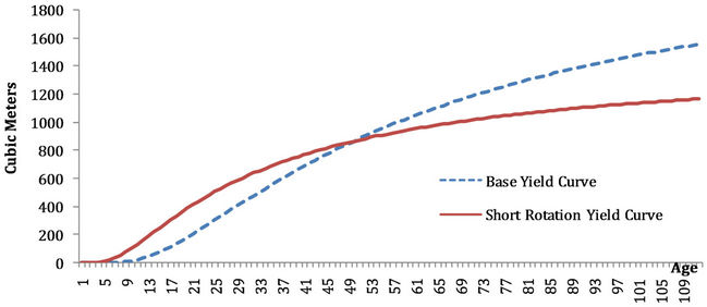
Figure 2. Wood yield curves.
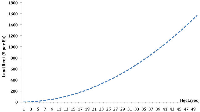
Figure 3. Constant elasticity land supply curve (land supply elasticity: 0.5).
allowed to adapt to facilitate meeting the intertemporal demand in an economically efficient manner. This is the stylized Base Case model from which the subsequent scenarios are developed. It also gives the reader an idea of how demand will affect the forest. The Base Case results are presented in Figures 4-7, for an initial 16 million ha forest. If the baseline demand is assumed to be constant at a low level compared with the forest size, Figure 5 shows the regulated forest area declining from 16 million ha to about 6 million ha over a period of almost 40 years. However, if the demand is growing (e.g., 2 percent per year over 40 years), the area of forest expands through that 40-year period. Thus, under management, the commercial forest adjusts over time to the demands placed upon it. For the constant demand, the initial 16 million ha is harvested over time, however, since only about 6 million ha is needed to meet the constant low level of anticipated demand and only that reduced amount of area is reforested. The remaining 10 million ha now falls out of the regulated forest and is assumed to be available for non forest uses after this area has been harvested. However, for the increasing demand situationthe area of forest is expanded to about 35 million ha in the face of rising prices and harvests (Figures 5-7).
A major lesson is that if demand is less than the sustainable harvest potential of the forest, the wood price will decline and with it the forest area and forest carbon. If, however, demand is greater than the sustainable harvest of the forest, prices will rise, the forest area will expand to meet the increasing demand, and in the process it will capture more forest carbon.
4.2. The Scenarios
In the two scenarios reported the level of initial demand is set just adequate to fully utilize the existing forest. When the rate of growth of demand is increased by some amount—reflecting, say, increased demand for biomass energy as renewables increasingly replace fossil fuels— the forest system adapts. As demand changes, the system converges to a new equilibrium path consistent with that demand and generates new intertemporal price, harvest, and forest area paths. Scenario 1 examines the effects of different levels of demand increase, and Scenario 2 ex
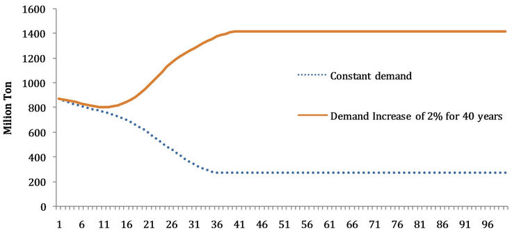
Figure 4. Base case: Carbon capture path. Note: Start with 16 million hectares in 32 equal age classes; base yield function; constant land rent.
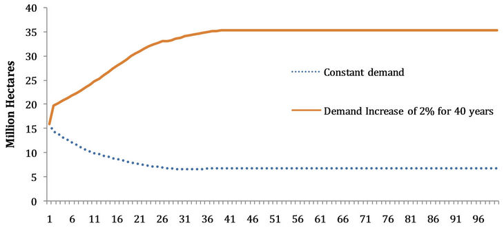
Figure 5. Base case: Forest area path. Note: Start with 16 million hectares in 32 equal age classes; base yield function; constant land rent.
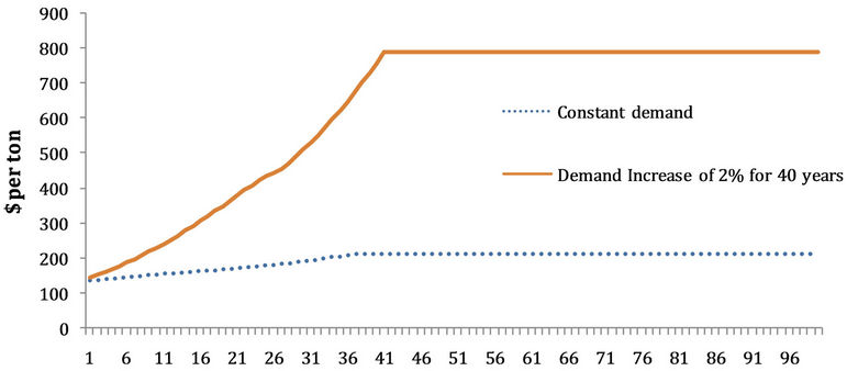
Figure 6. Base case: Wood biomass price path. Note: Start with 16 million hectares in 32 equal age classes; base yield function; constant land rent. The price axis is an index and indicates relative not absolute price level changes.

Figure 7. Base case: Harvest path. Note: Start with 16 million hectares in 32 equal age classes; base yield function; constant land rent.
amines the effects on the forest system of the reduced availability of land for conversion to forests as captured by a more inelastic supply of land available for conversion to forest.
Three other scenarios are examined but not presented in the figures. These are Scenario 3 that examines the effects of reducing the rotation length by using a fastgrowing tree species; Scenario 4 that examines the behavior of forests and carbon for the case of a declining demand for biomass energy; and Scenario 5 that examines the effect of increased bioenergy demand when facing a fixed forestland base—that is, zero supply elasticity, somewhat like in the Manomet study.
4.2.1. Scenario 1: Alternative Demands
Scenario 1 explores the effects of alternative anticipated demand growth rates on an initial forest in equilibrium. These results show that as higher demand is anticipated, the higher will be the time path of wood prices, forest area, harvest levels, and forest carbon stocks (Figures 8-11).
This scenario examines three levels of demand for a regulated forest of about 6 million ha and 28 age classes. This size forest is consistent with the size required for the long-run equilibrium for the level of constant demand chosen for this illustrative case. Demand is set at a given constant level indefinitely, representing a situation where only a modest amount of wood is used for bioenergy and this condition has been in effect for some time. We can view this demand as consistent with the pre-wood biomass era. The forestland supply curve is infinitely elastic at a $200 rental price. These figures provide the 100-year time path for the constant demand level. As Figure 8-11 show, these levels remain constant over the approximately 100-year period examined.
The two higher-demand growth scenarios posit that

Figure 8. Scenario 1: Carbon capture path. Note: Start with 6 million hectares in 28 equal age classes; constant land rent; base yield function.
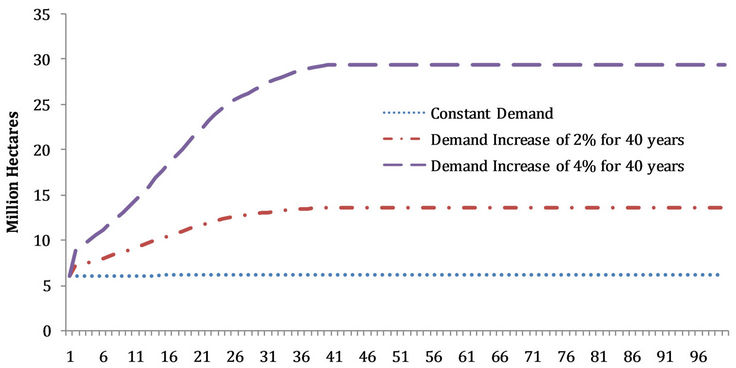
Figure 9. Scenario 1: Forest area path. Note: Start with 6million hectares in 28 equal age classes; constant land rent; base yield function.
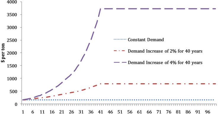
Figure 10. Scenario 1: Wood biomass price path. Note: Start with 6 million hectares in 28 equal age classes; constant land rent, base yield function. The price axis is an index and indicates relative not absolute price level changes.
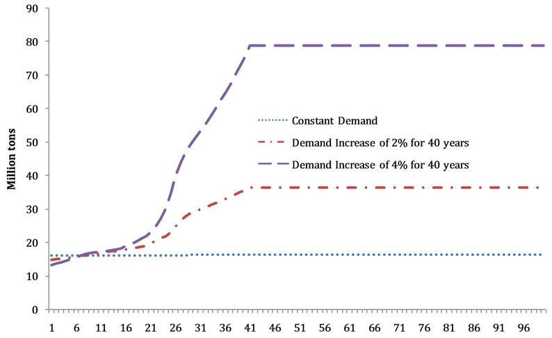
Figure 11. Scenario 1: Harvest path. Note: Start with 6 million hectares in 28 equal age classes; constant land rent; base yield function.
demand increases at a rate of 2 percent and 4 percent per year for 40 years and then remains at this level indefinitely. As is clear in Figures 8-11, the volumes of carbon captured, forest area, biomass wood price, and harvest levels all increase over the 40-year period of rising demand and then stabilize around year 40 at the higher levels.
4.2.2. Scenario 2: Land Supply Constraints
Scenario 2 (Figures 12-15) examines the effects on the forest when the land available to convert to forest is constrained. In this case the land supply elasticity is set at 0.5, indicating that land is available only at an increasing cost. Thus, land available for forest expansion is now less price responsive, with an elasticity of 0.5 throughout. This elasticity indicates that land supply curve is rising rather sharply as new land is added to the regulated forest to provide for increased production. The rising land prices are expected to choke off forest expansion to a degree.
For this case the initial conditions are modified to provide an initial equilibrium state for 9.69 million ha, divided into 28 equal age classes, with 370,000 ha in each class. As in the earlier scenario, this initial forestland area is consistent with the constant demand condition butis larger than in Scenario 1 because the supply conditions are different. The long-term price then peaks and stabilizes at a high level. In the index it is 850 or 4200 for the high demand scenarios driven by a yearly demand increase rate of 2 percent (or 4 percent). Note that in the earlier years, the harvest path is lower for the two cases where the level of demand is increasing over time than for the constant demand situation (Figure 15). This reflects optimizing behavior and rational expectations by managers, who delay harvests until prices have been raised. Note that simultaneously with the increasing rate of demand growth, the area of forest continues to increase despite rising land costs. The forest carbon path increases in the early years, reaches a peak, and declines until it stabilizes after about 45 years. Thus, for those two intervening decades there are net carbon releases to the atmosphere. However, even in its decline the forest carbon capture for increased wood biomass demand is always greater than that for the constant demand. Thus, the increased demand does not reduce total forest carbon in either the short or the long term compared with the constant demand case.
Finally, the other scenarios, whose figures are not presented here, show, for example, that selecting a species that shortens the rotation does not change the fundamental dynamics of the system (Scenario 3). Scenario 4 demonstrates the effects of a gradually declining demand on the basic forest system. In this case, not surprisingly, the forest contracts as does the carbon stock. Scenario 5 approximates the conditions assumed in the Manomet study, where the area of forest is fixed and is not allowed to expand. If the forest is a regulated forest, however, then the stock of wood and associated carbon rise as harvests are withheld and volumes allowed to build-up in anticipated of higher future prices. Once demand has stabilized in year 40, the stocks and harvests fall back to a steady-state sustainable level.
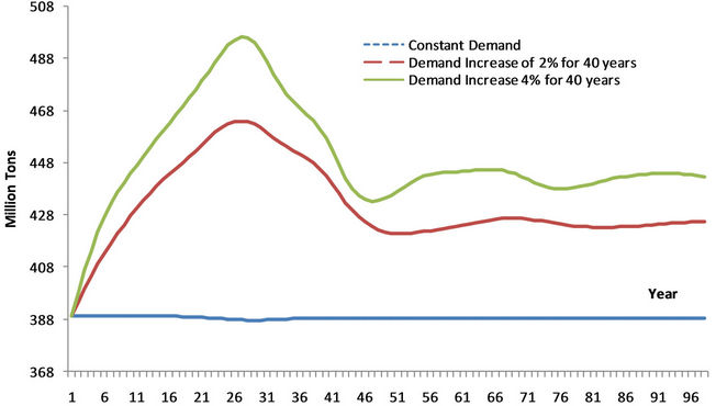
Figure 12. Scenario 2: Carbon capture path. Note: Start with 9.69 million hectares in 28 equal age classes; land supply elasticity of 0.5; base yield function.

Figure 13. Scenario 2: Forest area path. Note: Start with 9.69 million hectares in 28 equal age classes; land supply elasticity of 0.5; base yield function.
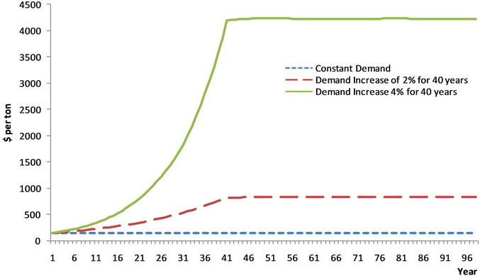
Figure 14. Scenario 2: Wood biomass price path. Note: Start with 9.69 million hectares in 28 equal age classes; land supply elasticity of 0.5; base yield function. The price axis is an index and indicates relative not absolute price level changes.
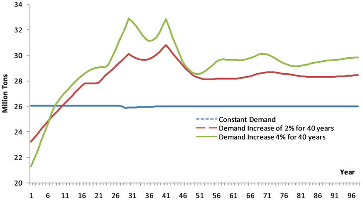
Figure 15. Scenario 2: Harvest path. Note: Start with 9.69 million hectares in 28 equal age classes; land supply elasticity of 0.5; base yield function.
5. Summary of Results and Some General Findings
Scenario 1 explores the effects of alternative anticipated demand growth rates on an initial forest in equilibrium. The results show that the higher the anticipated demand, the higher will be the time path of wood prices, forest area, harvest levels, and forest carbon stocks.
The Base Case and Scenario 1 have assumed availability of unlimited supplies of forestland at a constant price. Scenario 2 changes the assumption regarding the supply curve so that it has an elasticity of 0.5 throughout. This elasticity indicates that the land cost supply curve will rise as new land is added to the regulated forest to provide for increased production. The rising land costs choke off forest expansion to a degree. As in Scenario 1, the amount of forestland and carbon captured is constant for the constant demand scenario while increasing for both the higher demand scenarios. The long-term price is higher for the high demand scenario. Also, the harvest path is lower for the two cases where the level of demand is increasing over time. This reflects optimizing behavior and rational expectations: managers delay harvests until prices have risen. As the rate of demand growth increases, the area of forest and the forest carbon captured also increase, despite rising land costs. Other scenarios have been run but the figures are not presented here. But, the results are consistent in that forests expand in the face of rising anticipated demand and fall in the case of anticipated declining demand.
Where the initial conditions begin at a preexisting long-term equilibrium, an anticipated increase in the demand for wood biomass for a significant period (here, 40 years) will result in an increase in the size of the forest area, the harvest level, the stock of carbon, and the price of the biomass. In all cases examined, an anticipated long-term (40-year) increase in demand and harvest, stabilizing at the higher level, does not reduce forest carbon—even in the short run. This suggests that under many conditions, forests can supply wood for biomass energy without compromising their ability to capture and hold carbon. The anticipated overall increase in demand for wood would give managers incentive to increase the forest stock and with it the associated forest carbon. Finally, the model results have demonstrated that even if inelastic supply limits forest expansion, the general rule still holds: forest growth will offset the higher harvests, and an increase in anticipated demand will increase the carbon stock.
Where there is a nonequilibrium starting condition, some short-term forest carbon losses can occur. A nonequilibrium or a situation sharply different from the earlier equilibrium can affect whether the size and volume of the forest and its carbon increase or decrease initially. A spike in wood demand can reduce forest carbon initially, but expansion of the forest would reverse this in a relatively short period. Only a negative change in anticipated longer-term demand will reduce the size of the forest and its associated carbon stock.
6. Discussion
This paper addresses the carbon implications of using wood biomass as a substitute for fossil fuels. The Manoment study suggested that a full offset of carbon releases would require that the live wood used as biomass energy to substitute for fossil fuel be totally regrown before the carbon releases would be offset. For a mature forest stand in isolation, this would require decades and perhaps centuries. However, forest management does not involve simply harvesting mature stands and replanting them in isolation. Rather, forest managers respond to markets and simultaneously regulate multiple stands in anticipation of future market conditions. Indeed, the market coordinates wood use and forest management across many stands and ownerships. Thus, the regulated forest need not be managed by a single individual; multiple managers and forests are directed by market signals. This intertemporal management process for the forest system is captured by a dynamic optimization approach, whereby the entire intertemporal system is modeled and solved simultaneously, with the specified future conditions directly affecting current decisions.
A “forward-looking” rational expectations approach is now commonly used in forestry projections: one would expect future anticipated prices to be incorporated in current management decisions. Applying this approach to wood biomass for energy, this study demonstrates that managers in such a system would, on average, anticipate increases in the future demand and adjust their management, including forest size and harvests, accordingly. The model allows adjustments of only forest size and harvest levels; in the real world the managers also use additional silvicultural practices, such as fertilizer and genetics, to assist in the adaptation.
Although we find that carbon emissions associated with wood biomass energy ought to be viewed as offset in the short term, one question is whether the increased demand for wood biomass energy is expected to continue long enough to justify the appropriate adjustments in forest practices. A short surge in demand is unlikely to result in forest expansion.
It may be argued that many individual forests are not regulated. Collectively, however, the global forest system fits well into the model paradigm. The underlying forest production conditions, while they vary by region, are well known. Profit-maximizing forest managers will respond similarly to global markets, which in forest resources are well established. Planted and managed natural forests respond to market conditions, which have become well integrated. Biomass energy will draw, in part, on these same markets and presumably be reflected in investments that anticipate economic returns.
Finally, it should be noted that there may be a longterm trend of forestland conversion to non-forest land uses. This trend is due not to timber harvesting for industrial wood or wood biomass but largely to alternative land uses, such as agriculture. The phenomenon, however, does not provide any direct information for the question at hand—the effect of forest harvests for biomass energy on the net carbon footprint.
7. Conclusion
Our results suggest that the forest stock for a commercial regulated forest system will generally expand in the face of increasing demand as the forest expanding effects of the additional market derived investments in the forest stock exceed the forest contracting effects of the increased harvests. In the case of decreasing demand the forest will contract as investments in the forest are reduced and land is withdrawn from managed commercial forestry. Our analysis shows that the effect of wood biomass use on forest carbon is complex and counterintuitive. We observe that market driven commercial forests are not static. For a managed regulated forest with foresight, an anticipated substantial increase in future demand will not reduce forest carbon but rather, as forest management activities respond, increase the forest and forest carbon. This result occurs when forest managers are driven by economic returns on their forest investments. Our approach assumes that commercial forests harvested for wood biomass are market driven and return to pre harvest conditions as economic conditions dictate. We argue that these results occur not only for an individual commercial forest but also for a national and international forest system that is interconnect by a common global market to which commercial managers react. Market forces dictate that decisions in one forest will affect decisions in others. In summary, this analysis suggests that for a dynamic, forward-looking forest generating an economic commodity like wood biomass in response to market forces, the pressures to reduce the forest stock are offset by economic forces to increase that forest stock and, with it, forest carbon.
REFERENCES
- Intergovernmental Panel on Climate Change, “IPCC Guidelines for National Greenhouse Gas Inventories, Vol. 4: Agriculture, Forestry and Other Land Use,” IPCC, Geneva, 2006.
- B. Lippke, et al., “Letter to the Congress 12 May 2010,” 2010.
- W. Schlesinger, et al., “Letter to the Congress 20 July 20 2010,” 2009.
- Manomet Center for Conservation Science, “Biomass Sustainability and Carbon Policy Study,” Manomet Center for Conservation Science, Manomet, 2010. http://www.manomet.org/sites/manomet.org/files/Manomet_Biomass_Report_Full_LoRez.pdf
- R. W. Malmsheimer, J. L. Bowyer, J. S. Fried, E. Gee, R. L. Izlar, R. A. Miner, I. A. Munn, E. Oneil and W. C. Stewart, “Managing Forests Because Carbon Matters: Integrating Energy, Products, and Land Management Policy,” Journal of Forestry, Vol. 109, No. 17, 2011, pp. S35-S39. http://www.safnet.org/documents/JOFSupplement.pdf
- T. Searchinger, R. Heimlich, R. A. Houghton, F. Dong, A. Elobeid, J. Fabiosa, S. Tokgoz, D. Hayes and Yu. TunHsiang, “Use of US Croplands for Biofuels Increases Greenhouse Gases through Emissions from Land-Use Change,” Science, Vol. 319, No. 5867, 2008, pp. 1238-1240. doi:10.1126/science.1151861
- T. D. Searchinger, S. P. Hamburg, J. Melillo, W. Chameides, P. Havlik, D. M. Kammen, G. E. Likens, R. N. Lubowski, M. Obersteiner, M. Oppenheimer, G. P. Robertson, W. H. Schlesinger and G. D. Tilman, “Fixing a Critical Climate Accounting Error,” Science, Vol. 326, No. 5952, 2009, pp. 527-528. doi:10.1126/science.1178797
- J. Fargione, J. Hill, D. Tilman, S. Polasky and P. Hawthorne, “Land Clearing and the Biofuel Carbon Debt,” Science, Vol. 319, No. 5867, 2008, pp. 1235-1238. doi:10.1126/science.1152747
- R. A. Sedjo and B. Sohngen, “Wood as a Major Feedstock for Biofuel Production in the US: Impacts on Forests and International Trade,” Journal of Sustainable Forests, forthcoming, 2012.
- J. F. Muth, “Rational Expectations and the Theory of Price Movements,” In: The New Classical Macroeconomics, Vol. 1: International Library of Critical Writings in Economics, Elgar, Aldershot, 1992, pp. 3-23.
- T. Takayama and G. G. Judge, “Spatial and Temporal Price and Allocation Models,” North Holland Press, Amsterdam, 1971.
- R. A. Sedjo and K. S. Lyon, “The Long-Term Adequacy of World Timber Supply,” RFF Press, Washington DC, 1990, p. 220.
- B. Sohngen, R. Mendelsohn and R. Sedjo, “Forest Management, Conservation, and Global Timber Markets,” American Journal of Agricultural Economics, Vol. 81, No. 1, 1999, pp. 1-13. doi:10.2307/1244446
- D. M. Burton, B. A. McCarl, D. Adams, R. Alig, J. Callaway and S. Winnet, “An Exploratory Study of the Economic Impacts of Climate Change on Southern Forests,” Proceedings of the Southern Forest Economics Workshop, Savannah, 27-29 March 1994.
- D. M. Adams, R. J. Alig, J. M. Callaway, S. M. Winnett and B. A. McCarl, “The Forest and Agricultural Sector Optimization Model (FASOM): Model Structure, Policy and Applications,” Res. Pap PNW-RP-495. USDA Forest Service, Pacific Northwest Experiment Station, Portland, 1996.
- R. J. Alig, D. M. Adams, J. M. Callaway, S. M. Winnett and B. A. McCarl, “Assessing Effects of Mitigation Strategies for Global Climate Change with an Intertemporal Model of the US Forest and Agriculture Sectors,” Critical Reviews in Environmental Science and Technology—Economics of Carbon Sequestration in Forestry, Vol. 27, 1997, pp. S97-S111.
- D. M. Adams and R. Haynes, “The 1980 Softwood Timber Assessment Market Model: Structure, Projections, and Policy Simulations,” Forest Science, Vol. 22, No. 3, 1980.
- B. Sohngen and R. Sedjo, “A Comparison of Timber Market Models: Static Simulation and Optimal Control Approaches,” Forest Science, Vol. 44, No. 1, 1998, pp. 24-36.