Smart Grid and Renewable Energy
Vol.2 No.1(2011), Article ID:4033,9 pages DOI:10.4236/sgre.2011.21002
Probabilistic Load Flow Considering Correlation between Generation, Loads and Wind Power
![]()
Departamento de Enxeñería Eléctrica, Universidade de Vigo, Vigo, Spain.
Email: {dvillanueva, afeijoo, pazos}@uvigo.es
Received December 27th, 2010; revised January 11th, 2011; accepted January 16th, 2011.
Keywords: Correlation, Monte Carlo Simulation, Probabilistic Load Flow, Wind Power, Wind Farm
ABSTRACT
In this paper a procedure is established for solving the Probabilistic Load Flow in an electrical power network, considering correlation between power generated by power plants, loads demanded on each bus and power injected by wind farms. The method proposed is based on the generation of correlated series of power values, which can be used in a MonteCarlo simulation, to obtain the probability density function of the power through branches of an electrical network.
1. Introduction
1.1. Probabilistic Load Flow
The Probabilistic Load Flow (PLF) analysis consists of obtaining the system state and power flows in an electrical power network considering the probabilistic nature of the power injected by generators and consumed by loads. It was first proposed by Borkowska in 1974 [1], and widely developed by Allan [2-12]. It has been applied to management, and also to short-term and long-term electrical network planning.
In order to solve the PLF, analytical and simulation methods have been proposed since 1974. The first methods to appear were based on the convolution of the PDF of two variables, in order to obtain the one corresponding to the sum of both. These processes are based on some approximations made in the equations that relate power and voltage in an electrical network, such as those applied to DC Load Flow [4] or AC Load Flow [6,12], to obtain the sensitivity coefficients. The problem has been alternatively solved by means of linearizations around the operating point [5,6,10,13,14] or even around several of these [8]. Second order approximations have also been used [15] or even n-order ones [16]. Lately, the GramCharlier expansion [17,18] was used. However, the Monte Carlo (MC) simulation is sometimes the proposed method [13,19,20], due to additional considerations as the network configuration, voltage control devices or the addition of Wind Turbines (WT).
Generally, the probabilistic nature of the injected power and loads is considered, but sometimes the unpredictability of the branch impedances is also taken into account [14] or the possible network configurations [9,21]. The correlation between injected powers, loads and also between injected power and loads due to meteorological or social factors has also been considered [10,11,13].
The wind power integration has been widely implemented in the PLF [18,19,22-26].
1.2. Correlation between Generation, Loads and Wind Power
The existence of correlation, or even dependence, between generation and load (i.e., between injected and consumed power) is intuitive. But it can be said that it is completely necessary for the stability of the network.
The generation has to supply the demanded load, so a full dependence between the sum of all the loads and the sum of all the generations in a system can be obviously assumed.
The losses in the network lower this dependence slightly. Although the consideration of several supply plants and loads involves this dependence being reduced, it cannot be avoided, and influences in the results of the PLF.
Dependence between loads operates in a similar way. Environmental or social factors make them increase or fall almost simultaneously. Therefore, there is a certain degree of dependence between them.
The dependence between the power produced by several power plants exists because of the need to balance the system power. This balance is achieved when several circumstances are considered such as economic dispatch, redispatch and load shedding.
The power provided by each power plant depends on its type. The power generated by the base load units essentially depends on their forced outage rates. The power generated by intermittent and peaking units depends on the total system load, on the unit unavailability and also on the dispatcher activity function.
The dependence shown by wind power is widely known, and is deduced from the analysis of the dependence between wind speed at different locations, although this dependence is reduced as long as the distance between them increases [27].
Moreover, the dependence between Wind Farm (WF) generation and other power plants exists, since they all have to fulfill the total load demand and as more wind power is generated, less power is needed from the other plants. In this case there is an inverse dependence.
The dependence between wind power and loads can be understood by considering that the wind power, as it is originally produced by the sun, reaches its higher values throughout daylight, and its lower ones during the night. These stages are almost simultaneous with the load variations.
The correlations explained above are given through the correlation coefficient. If dependence is assessed in terms of correlation, then we can say that correlation coefficient values close to 1 mean strong dependence, close to –1 mean strong inverse dependence, and close to 0 mean small dependence.
1.3. State of the Art
In [11] the correlation is introduced in the PLF problem, obtaining Probability Density Function (PDF) for the correlated variables, and performing the analytical PDF method based on convolution, which is not correct, because it does not assure the correlation of the input data, just the right PDF of each one.
Later, [10] introduces the linear relationship between correlated variables in order to solve the PLF problem, utilizing the method of linearization around the expected value, which can produce good results in case of high correlation but does not work properly when the correlations are lower.
And [13] utilizes the method proposed in [10], but adding the multilinearizations, which have the same drawbacks as before.
Correlation between wind power has been analyzed on its own [28] based on methods of simulation of correlated wind speed [29-31], on prediction [32], and also applied to different fields [26,33,34].
In this paper a method is presented to consider the correlations between generation, loads and wind power, therefore, correlation data have to be provided or estimated in order to obtain results for the PLF problem.
2. The Proposed Method
The goal of the PLF is to obtain the PDFs or Cumulative Distribution Function (CDF) of the system state and power flows in an electrical power network, knowing the probabilistic nature of the power injected and loads demanded, and the correlation between them. Therefore, the input data will be the probabilistic distribution (PDF or CDF) of all the power plants, loads and WFs included in the electrical network and the correlation coefficients (correlation matrix).
The proposed method consists of the following steps:
1) For each power plant, load and/or WF in the electrical network, a number (N) of samples of power values are generated, in order to obtain m vectors, considering the probabilistic nature of the values.
2) These vectors, considering their random origin, have a correlation matrix that must not be the same as the one provided. These data are dealt with in order to fulfill this correlation matrix, but maintaining the features of the probability distribution of each one of the m vectors.
3) Utilizing these data, the Load Flow is solved for each one of the N samples of input data, i.e., a MC simulation is performed, generating the PDFs of the bus voltages and power flows.
All these steps are explained in detail in the following sections.
2.1. Generation of Samples
First, it is necessary to state that the number of vectors to be generated does not have to coincide with the number of buses in the electrical network. This number, m, has to be the sum of the elements whose correlation by pairs is considered, so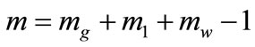 , where mg is number of power plants, ml the loads and mw the WFs. The slack bus is removed as it is not an input data. Therefore a correlation matrix of m × m elements has to be provided as input data.
Each element, power plant, load or WF, has a probabilistic nature relating their power values, although there are important differences between them, so they are treated separately.
2.1.1. Power Plant Generated Power
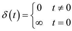
A power plant is made up of several generators, which can each be described probabilistically by means of a binomial distribution considering its forced outage rate. Therefore, the power plant is described by a multinomial probability mass function, that can be expressed as a PDF utilizing the delta of Dirac function, as in (1).
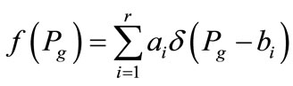 (1)
(1)
Where Pg is the power, ai is the probability associated to power value bi, and r is the number of discrete values for power.
2.1.2. Load Demand Power
Each load is probabilistically described by a normal distribution, with a PDF described such as in (2).
 (2)
(2)
Where Pl is the power, µ is the mean value and σ is the standard deviation.
2.1.3. Wind Farm Generated Power
In the WF case, the PDF has to be deduced as explained in [35] and in most cases can be approximated by equation (3).
 (3)
(3)
Where Pw is the power, C and k are the Weibull parameters of the wind speed in the location of the WF, UCI, UR, UCO, are the parameters of the WTs installed in the WF, PR is n times the rated power of the WTs, n is the number of WT and C’, k’ and γ’ have the values shown in (4).
 (4)
(4)
According to [35] if the WF does not fulfill the requirements to be represented by the PDF shown in (3), another method is proposed. To obtain the PDF of a WF is beyond the aim of this work.
In order to generate the samples of power injected by a power plant, load or WF, an MC simulation utilizing their respective PDFs can be performed, generating N samples for each of the m elements.
2.2. Correlation between Powers
The values for each correlation coefficient of the m × m matrix depends on the type of elements involved in each pair (generation/generation, load/load, wind power/wind power, generation/load, generation/wind power or load/ wind power) and on the degree of dependence between them. These values can vary from –1 to 1 and should be calculated from known data or, in case there are no available data, estimated on the basis of the information provided.
In order to convert the N × m samples generated in the last step, in N × m samples with the correlation coefficients set by the m × m correlation matrix, M, maintaining the probabilistic distribution of each vector, one of the methods to perform this operation should be utilized.
These methods are described in [29-31]. Based on its simplicity, speed and proper results, the method used here is the one described in [30], but any of the others can be used in substitution.
In this method, Spearman rank correlation coefficients are used instead of the conventional Pearson correlation ones, so the matrix M has to be provided considering this feature and the results obtained operate in the same way. The use of Spearman rank correlation coefficients does not constitute a problem different from the own use of this definition for the coefficients instead of other parametric definitions, and the method described in [30] gives better results than those obtained when using Pearson correlation coefficients [29,30].
This method consists of generating m uniform samples of N elements and adequately operating them by means of the Cholesky decomposition of the given correlation matrix, making it possible for the m uniform samples of N elements to have the correlation values provided in the correlation matrix. The m × N uniform samples have been ordered in the same way as the m × N different-type of samples generated in the last step of the method, so they are reordered in that way. The resulting m × N samples of different types fulfill the correlation matrix M and maintain the probabilistic distribution of each of the m vectors of samples.
2.3. Monte Carlo Simulation
Starting with the correlated data, the next step consists of defining the injected or consumed power on each bus. For each bus and sample, it is necessary to add the powers provided by the power plants and WFs at the bus, and subtracting the power demanded by each load at the same bus. This step converts the m × N samples in s × N, where s is the number of buses minus 1.
After this it is necessary to solve N Load Flows. In order to obtain the desired results, any of the methods utilized in a Load Flow can be valid, the difference lies in the approximation level.
The method proposed here suggests the DC Load Flow due to its simplicity, easy implementation and good results provided. However, the DC Load Flow can be changed to any of the other known methods (AC Load Flow in any of its formulations, Newton-Raphson, Gauss-Seidel, etc.).
The DC Load Flow consists of the calculation of sensitive coefficients, one for each bus (except for the slack one), which relate the power flow through any branch, with the power injected/consumed in/by each bus. These coefficients just depend on the network configuration and are obtained using (5).
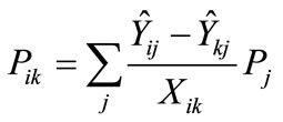 (5)
(5)
where Pik is the power from bus i to bus k, Pj is the power injected/consumed in/by bus j, Ŷij and Ŷkj are elements of the inverse matrix Ŷ, defined in (6).
 (6)
(6)
Once the sensitive coefficients are calculated, the computation is repeated N times, in order to obtain N results for each line.
The results can be grouped in intervals and their relative frequencies will be used to constitute a PDF as a final result.
3. Case Study
The proposed method has been tested in the IEEE 96- RTS system, having used the values in Tables 1-3 and IV, and considering two WFs injecting power in the system, through buses 107 and 113, both modeled according to (3) and with rated powers of 100 and 300 MW respectively. The system has been represented in Figure 1.
In Table 1 the composition of each power plant is given. In Table 2 the features of each unit are provided. Slack bus is bus 1. The mean values and standard deviation of the loads are given in Table 3. Table 4 provides branch data.
The proposed method has been implemented with help of MATLAB software. N has been fixed to 10,000.
Results obtained for power through lines 102-106 and 108-110 have been presented in Figures 2 and 3. In these figures, the case simulated with no correlation is shown by a dotted line; high correlation (0.9) between power plants by means of a dash-dot one; high correlation between loads by a dashed line; high correlation between
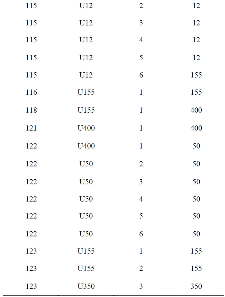

Table 1. Data of Power Plants at Each Bus in IEEE 96-RTS.
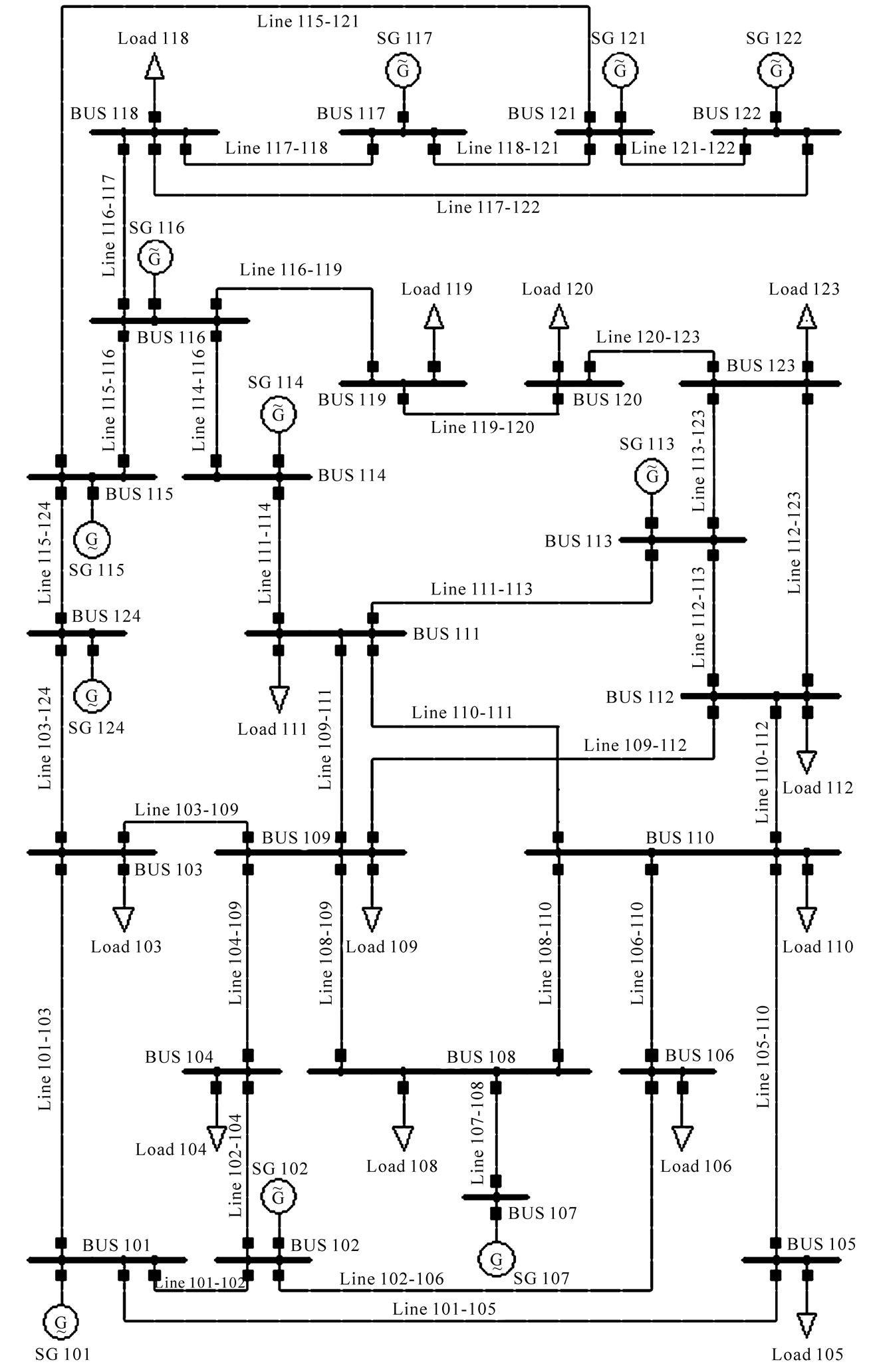
Figure 1. IEEE 96-RTS schematic drawing.
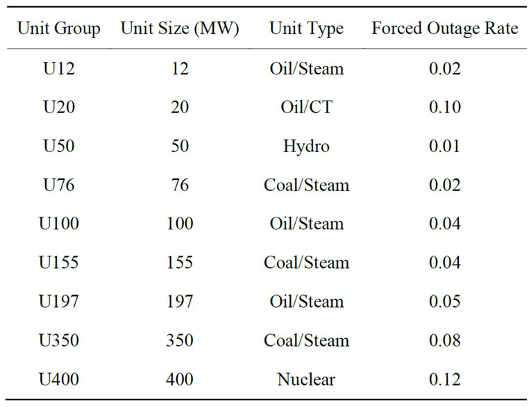
Table 2. Unit data for power plants.
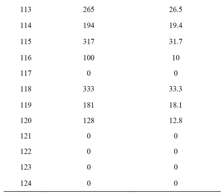

Table 3. Bus Loads in IEEE 96-RTS.
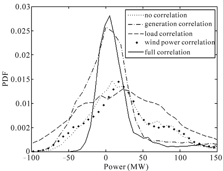
Figure 2. PDF of the power through line 102-106 in IEEE 96-RTS.
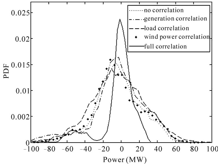
Figure 3. PDF of the power through line 108-110 in IEEE 96-RTS.
WFs by points; and high correlation between all of them by a solid line, in order to show the more extreme cases.
First, when no correlation is considered, the result is the same as a MC simulation with no dependence, and this constitutes the reference in order to compare the results with other conventional methods that are utilized and considered valid. In case of line 102-106 the correlation between power plants has great influence, and increases the probability to have certain values for power flows; in line 108-110 this correlation does not have great influence. Again, for load correlation, the power flow through line 102-106 decreases its probability to present centered values and almost no influence in line 108-110. When wind power correlation is considered, there is a slightly modification in the PDF of line 102-106 and almost no modification in line 108-110. And finally, when high correlation between all of them is taking into account, it has great influence in the PDF of the power
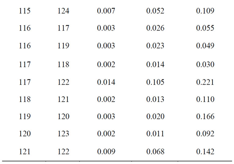

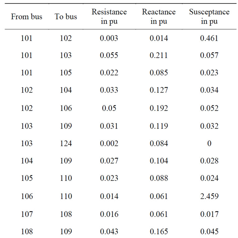
Table 4. Line Parameters of the IEEE 96-RTS.
through both lines, making it sharper, which is repeated for all the lines of the network.
It can be said that the line 102-106 is greatly influenced by any type of correlation whereas line 108-110 is just influenced is case of full correlation. The reason is the network configuration, for example, in bus 102 there are four units connected and in case of high correlation among them the result may be influenced, in the other hand, line 108-110 has no units connected so the correlation has less influence in the results.
4. Conclusions
A method has been proposed, for statistically obtaining the power flow through lines in an electrical network, given the statistical nature of the injected power, loads and wind power and considering the correlation between them. It is based on the MC simulation and applied under correlated input data conditions.
Previous methods considering correlation do not provide good results, or their approach is partially wrong, as shown in Section 1.3.
The main concern about the MC method is the need for large number of simulations, which is very time-consuming. However, the time is reduced utilizing the DC Load Flow instead of iterative Load Flow methods.
Therefore, the great advantages of this method are its simplicity, speed, easy implementation and good approximation of the results. It also includes the possibility to change the procedure of steps 2 and 3 in order to increase the accuracy of the results, reducing its speed.
Possible applications for this method are the following:
1) Introducing the dependence factor in the PLF, providing more realistic results. All possible types of correlation are taken into account.
2) Observing the influence of future installation of WFs in an electrical power network, where correlation is critical in the PLF problem.
3) Predicting the influence of potential situations where environmental or social factors can cause synchronized load demands.
4) As long as the WFs are spread over the land, due to their dependence on the sun, the total correlation between injected power and loads is increased. With the proposed method, it is possible to consider this situation, which is not with former methods.
In order to schedule long-term maintenance operations, the influence of disconnect units or power plants from the network can be calculated considering correlation, which are more realistic results.
REFERENCES
- B. Borkowska, “Probabilistic Load Flow,” IEEE Transactions on Power Apparatus and Systems, Vol. PAS-93, No. 3, May-June 1974, pp. 752-755.
- R. N. Allan, B. Borkowska and C. H. Grigg, “Probabilistic Analysis of Power Flows,” Proceedings of the Institution of Electrical Engineers, London, Vol. 121, No. 12, December 1974, pp. 1551-1556.
- A. M. Leite da Silva, S. M. P. Ribeiro, V. L. Arienti, R. N. Allan and M. B. Do Coutto Filho, “Probabilistic Load Flow Techniques Applied to Power System Expansion Planning,” IEEE Transactions on Power Systems, Vol. 5, No. 4, November 1990, pp. 1047-1053.
- R. N. Allan, C. H. Grigg and M. R. G. Al-Shakarchi, “Numerical Techniques in Probabilistic Load Flow Problems,” International Journal for Numerical Methods in Engineering, Vol. 10, No. 4, March 1976, pp. 853-860.
- R. N. Allan, A. M. Leite da Silva and R. C. Burchett, “Evaluation Methods and Accuracy in Probabilistic Load Flow Solutions,” IEEE Transactions on Power Apparatus and Systems, Vol. PAS-100, No. 5, May 1981, pp. 2539-2546.
- R. N. Allan and M. R. G. Al-Shakarchi, “Probabilistic a. c. Load Flow,” Proceedings of the Institution of Electrical Engineers, Vol. 123, No. 6, June 1976, pp. 531-536.
- R. N. Allan, A. M. Leite da Silva and R. C. Burchett, “Discrete Convolution in Power System Reliability,” IEEE Transactions on Reliability, Vol. R-30, No. 5, December 1981, pp. 452-456.
- R. N. Allan and A. M. Leite da Silva, “Probabilistic Load Flow Using Multilinearisations,” IEE Proceedings of Part C: Generation, Transmission and Distribution, Vol. 128, No. 5, September 1981, pp. 280-287.
- A. M. Leite da Silva, R. N. Allan, S. M. Soares and V. L. Arienti, “Probabilistic Load Flow Considering Network Outages,” IEE Proceedings of Part C: Generation, Transmission and Distribution, Vol. 132, No. 3, May 1985, pp. 139-145.
- A. M. Leite da Silva, V. L. Arienti and R. N. Allan, “Probabilistic Load Flow Considering Dependence between Input Nodal Powers,” IEEE Transactions on Power Apparatus and Systems, Vol. PAS-103, No. 6, June 1984, pp. 1524-1530.
- R. N. Allan, C. H. Grigg, D. A. Newey and R. F. Simmons, “Probabilistic Power-Flow Techniques Extended and Applied to Operational Decision Making,” Proceedings of the Institution of Electrical Engineers, Vol. 123, No. 12, December 1976, pp. 1317-1324.
- R. N. Allan and M. R. G. Al-Shakarchi, “Probabilistic Techniques in a. c. Load Flow Analysis,” Proceedings of the Institution of Electrical Engineers, Vol. 124, No. 2, February 1977, pp. 154-160.
- A. M. Leite da Silva and V. L. Arienti, “Probabilistic Load Flow by a Multilinear Simulation Algorithm,” IEE Proceedings of Part C: Generation, Transmission and Distribution, Vol. 137, No. 4, July 1990, pp. 276-282.
- C. L. Su, “Probabilistic Load-Flow Computation Using Point Estimate Method,” IEEE Transactions on Power Systems, Vol. 20, No. 4, pp. November 2005, 1843-1851.
- M. Brucoli, F. Torelli and R. Napoli, “Quadratic Probabilistic Load Flow with Linearly Modelled Dispatch,” Electrical Power & Energy Systems, Vol. 7, No. 3, July 1985, pp. 138-146.
- X. Li, X. Chen, X. Yin, T. Xiang and H. Liu, “The Algorithm of Probabilistic Load Flow Retaining Nonlinearity,” Proceedings of 2002 International Conference on Power System Technology, Kunming, Vol. 4, 10 October 2002, pp. 2111-2115.
- P. Zhang and S. T. Lee, “Probabilistic Load Fow Computation Using the Method of Combined Cumulants and Gram-Charlier Expansion,” IEEE Transactions Power Systems, Vol. 19, No.1, February 2004, pp. 676-682.
- J. Usaola, “Probabilistic Load Flow with Wind Production Uncertainty Using Cumulants and Cornish-Fisher Expansion,” International Journal of Electrical Power and Energy Systems, Vol. 31, No. 9, 2009, pp. 474-481.
- P. Jorgensen, J. S. Christensen and J. O. Tande, “Probabilistic Load Flow Calculation Using Monte Carlo Techniques for Distribution Network with Wind Turbines,” 8th International Conference on Harmonics and Quality of Power, Athens, Vol. 2, 14-16 October 1998, pp. 1146-1151.
- C. L. Su, “Distribution Probabilistic Load Flow Solution Considering Network Reconfiguration and Voltage Control Devices,” 15th Power Systems Computation Conference, Liege, August 2005.
- Z. Hu and X. Wang, “A Probabilistic Load Flow Method Considering Branch Outages,” IEEE Transactions on Power Systems, Vol. 21, No. 2, May 2006, pp. 507-514.
- N. D. Hatziargyriou, T. S. Karakatsanis and M. Papadopoulos, “Probabilistic Load Flow in Distribution Systems Containing Dispersed Wind Power Generation,” IEEE Transactions on Power Systems, Vol. 8, No. 1, February 1993, pp. 159-165.
- N. D. Hatziargyriou, T. S. Karakatsanis and M. P. Papadopoulos, “The Effect of Wind Parks on the Operation of Voltage Control Devices,” 14th International Conference and Exhibition on Electricity Distribution. Part 1. Contributions, London, Vol. 5, June 1997, pp. 1-5.
- N. D. Hatziargyriou, T. S. Karakatsanis and M. I. Lorentzou, “Voltage Control Settings to Increase Wind Power Based on Probabilistic Load Flow,” International Journal of Electrical Power and Energy Systems, Vol. 27, No. 9-10, 2005, pp. 656-661.
- P. Caramia, G. Carpinelli, M. Pagano and P. Varilone, “Probabilistic Three-Phase Load Flow for Unbalanced Electrical Distribution Systems with Wind Farms,” IET Renewable Power Generation, Vol. 1, No. 2, June 2007, pp. 115-122.
- J. Usaola, “Probabilistic Load Flow with Correlated Wind Power Injections,” Electric Power Systems Research, Vol. 80, No. 5, 2010, pp. 528-536.
- L. Freris and D. Infield, “Renewable Energy in Power Systems,” John Wiley & Sons, Chichester, 2008.
- D. Villanueva, A. Feijoo and J. L. Pazos, “Correlation between Power Generated by Wind Turbines from Different Locations,” Scientific Proceedings of the European Wind Energy Conferences, Warsaw, 2010, pp 183-185.
- A. Feijóo, J. Cidrás and J. L. G. Dornelas, “Wind Speed Simulation in Wind Farms for Steady-State Security Assessment of Electrical Power Systems,” IEEE Transactions on Energy Conversion, Vol. 14, No. 4, December 1999, pp. 1582-1588.
- A. Feijóo and R. Sobolewsky, “Simulation of Correlated Wind Speeds,” International Journal of Integrated Energy Systems, Vol. 1, No. 2, 2009, pp. 99-106.
- D. Villanueva and A. Feijóo, “A Genetic Algorithm for the Simulation of Correlated Wind Speeds,” International Journal of Integrated Energy Systems, Vol. 1, No. 2, 2009, pp. 107-112.
- G. Papaefthymiou and P. Pinson, “Modeling of Spatial Dependence in Wind Power Forecast Uncertainty,” Proceedings of the 2008 PMAPS, Mayagüez, May 2008.
- X. Lu, M. McElroy and J. Kiviluoma, “Global Potential for Wind-Generated Electricity,” Proceedings of the National Academy of Sciences of the United States of America, Washington, 2009.
- F. Vallée, J. Lobry and O. Deblecker, “System Reliability Assessment Method for Wind Power Integration,” IEEE Transactions on Power Systems, Vol. 23, No. 3, 2008, pp 1288-1297.
- D. Villanueva, J. L. Pazos and A. Feijóo, “Probabilistic Load Flow Including Wind Power Generation,” IEEE Transactions on Power Systems, 2011. (Accepted)
Appendix
Some expressions of the power PDFs use the known function called Dirac’s delta, about which a brief reminder is written here.
Dirac’s delta is a generalized function or density distribution function that can be defined in an informal way as follows:
 (A.1)
(A.1)
Although perhaps it is more correct to define it in these alternative ways:
 (A.2)
(A.2)
NOTES
*The financial support given by the autonomous government Xunta de Galicia, under the contract 08REM009303PR is acknowledged by the authors.