Communications and Network
Vol.5 No.3(2013), Article ID:35436,6 pages DOI:10.4236/cn.2013.53022
Enhancing Sentiment Analysis on Twitter Using Community Detection
Department of Computer Science, Houghton College, Houghton, USA
Email: *wei.hu@houghton.edu
Copyright © 2013 William Deitrick et al. This is an open access article distributed under the Creative Commons Attribution License, which permits unrestricted use, distribution, and reproduction in any medium, provided the original work is properly cited.
Received April 26, 2013; revised May 26, 2013; accepted June 26, 2013
Keywords: Community Detection; Twitter; Social Networks; Sentiment Analysis; SentiWordNet; Walktrap
ABSTRACT
The increasing popularity of social media in recent years has created new opportunities to study the interactions of different groups of people. Never before have so many data about such a large number of individuals been readily available for analysis. Two popular topics in the study of social networks are community detection and sentiment analysis. Community detection seeks to find groups of associated individuals within networks, and sentiment analysis attempts to determine how individuals are feeling. While these are generally treated as separate issues, this study takes an integrative approach and uses community detection output to enable community-level sentiment analysis. Community detection is performed using the Walktrap algorithm on a network of Twitter users associated with Microsoft Corporation’s @technet account. This Twitter account is one of several used by Microsoft Corporation primarily for communicating with information technology professionals. Once community detection is finished, sentiment in the tweets produced by each of the communities detected in this network is analyzed based on word sentiment scores from the well-known SentiWordNet lexicon. The combination of sentiment analysis with community detection permits multilevel exploration of sentiment information within the @technet network, and demonstrates the power of combining these two techniques.
1. Introduction
A social network is a relational structure comprised of entities (nodes) and the connections between them. Analysis of these structures can identify local and global relationships, locate influential entities, and reveal the dynamics of the network as a whole. Social networks were first investigated in the 1930’s. At that time they were called sociograms and were used to study interpersonal relationships. These structures were mathematically formalized in the 1950’s and methods using social networks became pervasive in the social and behavioral sciences in the 1980’s [1].
The study of social networks can be split into micro and macro levels. At the micro level, social network research typically begins with an individual or small group of individuals in a unique social context. The smallest and most simplistic network is one containing two entities, called a dyad. Research on these types of networks normally focuses on the structure or strength of the relationship. Investigating macro social networks normally focuses on the outcomes of interactions such as personal disagreements and economic or resource interactions over a large population. Network mapping is used quite often to track these changes in macro networks.
1.1. Community Detection
Because of the prevalence of social networks, community detection on these networks has become an important research topic. Using community detection, useful metadata about large scale networks can be captured. These communities represent relationships between entities and allow us to examine patterns that emerge in social media, publications, and a multitude of other types of networks. Community detection also allows for easy visualization of networks and their structure. In biological networks, communities signify functional modules in which members of a module act together to perform essential cellular tasks. In order to identify these modules, various forms of community detection have been used [2].
Community detection in networks is a challenging task because of the unknown number and varied sizes of communities within the network. Extremely large networks pose further computational difficulty in accurately detecting community structure. Despite these challenges, many methods for community detection have been developed and employed with varying levels of success. Though each of these methods successfully detects communities within a network, they all have distinct advantages and disadvantages. Since each method of community detection reveals the structure of the network in a different way, each technique is useful depending on the type of network being studied. Some of the most commonly used types of community detection include hierarchical clustering, modularity maximization, and spectral clustering [3]. Spectral clustering builds partitions in a network to create disjoint subsets within the vertices. This is useful for understanding graph data, but is not useful for detecting overlapping communities. Another downfall of spectral clustering is that this method requires knowing the number of communities a priori. Hierarchical clustering has the advantage of not requiring a predetermined number of communities. The two types of hierarchical clustering, agglomerative and divisive, allow for clusters to be made in either a top-down or bottom-up fashion. Edge “betweenness” has also been used as a form of community detection. Instead of trying to detect the most central edges in a graph, edge betweenness focuses on the least central edges and progressively removes them one by one in order to hone in on the most central edges [4]. Modularity maximization is another useful community detection technique which attempts to measure how well a given partition of a network compartmentalizes its communities [5].
1.2. Sentiment Analysis
Understanding the opinions of large groups of people is invaluable in many disciplines. Businesses need to gauge interest in their products and politicians determine their campaign platforms based on popular opinion. Traditionally, polling has been the standard method for gathering this information, but this is costly in terms of time, money, and manpower, and is difficult to distribute to large groups of people. An additional problem is that with traditional polling methods, respondents may not give accurate answers due to a variety of factors, such as misreporting or the influence of the surveyor [6]. Microblogging is a new and important alternative source of opinion data. Using social media platforms such as Facebook and Twitter, individuals can publish their ideas and distribute them very quickly throughout the network. By gathering information published in this way, researchers can acquire more accurate and widely representative data without concerns of survey bias. This computational method of gathering opinion from existing data is called sentiment analysis, and its two primary forms are classifying a statement as subjective or objective, or as expressing positive or negative sentiment [7]. The latter form is the focus of this paper. Besides public opinion collection, applications of sentiment analysis include automated review agglomeration, vendor website recommendations, automated advertising systems, information extraction, and many others [8].
Twitter is a particularly helpful tool for sentiment analysis, because Tweets are primarily public, while Facebook posts are generally restricted to friends. For this reason, the pool of relevant Tweets is much larger than for Facebook posts. In addition to the availability of tweets, the Twitter API makes data extraction a trivial operation [9]. However, the volume of data present on Twitter creates a significant challenge. The amount of Twitter data makes it important to be able to automatically determine which tweets are relevant and classify the data as positive or negative. Most people can read a tweet and evaluate its subjective content, but in massive data sets manual classification is unrealistic. Therefore it becomes important to have computer models which can automatically classify data.
There are two main families of sentiment analysis techniques, machine learning and semantic orientation. Machine learning sentiment analysis techniques use standard machine learning methods; a classification model is trained to distinguish between the different sentiment classes. Semantic orientation techniques involve creating a dictionary of subjectively meaningful words, and in some cases word modifiers, and using this dictionary to score a document’s subjective content [10]. Using such techniques enables much faster sentiment analysis, and makes it possible to perform sentiment studies on such large data sources as Twitter.
2. Materials and Methods
2.1. Dataset
The dataset used for this study consisted of data downloaded directly from the Twitter API. First, the Python library Tweepy (http://tweepy.github.com/) was used to crawl the social graph (friends and followers) of the Microsoft-owned account @technet. This account is used by Microsoft Corporation to communicate primarily with information technology professionals. The @technet account was chosen because data for this account were available from a previous study and its relatively small number of friends and followers permitted more rapid processing. All followers and friends of the @technet account who were following fewer than 600 others were gathered from the Twitter API. Filtering accounts following more than 600 others provided a way to reduce the number of large institutional accounts collected. This process ultimately created a social network of 1382 nodes in which all nodes were, at minimum, followers or friends of the @technet account.
After the @technet network had been crawled, the social graph for this account was constructed. The Python interface to the iGraph (http://igraph.sourceforge.net/) framework was used to create and manipulate the resulting graph object. This graph was constructed as a directed graph, with vertices representing users and edges representing connections amongthem. The resulting graph contained 1382 vertices, corresponding to the number of users collected from the social network of the @technet account, and 4834 edges.
Once the social network of the @technet account had been constructed, the second stage of data collection was initiated. This involved capturing all tweets created by users who were members of the @technet social graph. This time, the Twitter Streaming API was used in conjunction with the Java library Twitter4j (http://twitter4j.org). A total of 23,750 tweets were collected from users in the @technet social graph between January 2nd, 2013 and February 2nd, 2013. The tweet dataset resulting from this collection process is described in Table 1, and describes the number of tweets collected on each day.
2.2. Walktrap
The Walktrap community algorithm uses random walks
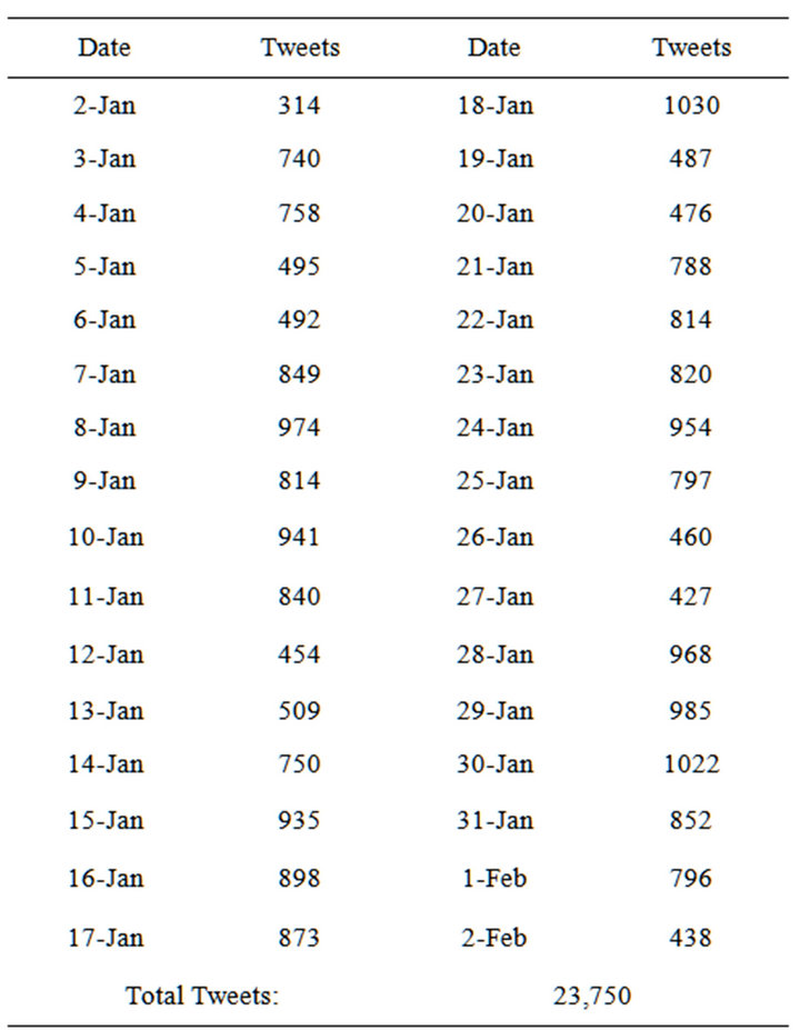
Table 1. Tweets collected per day.
to find the distance between two vertices in a graph. The search path of a grazing horse or the price of a company’s stock can be modeled as a random walk. Random walks on a graph tend to be trapped inside of the group of densely connected vertices. These random walks are used to define a measurement of the similarity between vertices and therefore are able to calculate a distance [11].
The variable r denotes a distance value between two nodes within a network. Larger distances signify that the two compared nodes are likely in separate communities, whereas smaller distances suggest that the two nodes are members of the same community. The probability 
measures the likelihood of the random walk moving from vertex i to j. Another value,  measures the same probability after t steps of the random walk. If two vertices i and j are in the same cluster, the probability
  will be very high. However, a high
  value does not necessarily mean that i and j are in the same community. The probability
  will be influenced by the degree d(j).
The walker has a better chance to go to vertices with a high degree.
The distance between i and j at step t,  , can be computed in time. The worst case scenario of running this Algorithm is time
  where m is the number of edges and n is the number of vertices. Most real world complex networks that are used are sparse networks and their time is
  and the most favorable situation is a balanced network
  where H is the height of the tree structure called a dendrogram [11].
2.3. Sentiment Analysis
After community detection had been performed on the friend/follower network associated with the @technet account, sentiment analysis was employed to analyze the sentiment expressed by users in each of the clusters over the 32 days in which tweets were collected. First, the tweets were divided by the cluster from which they originated. Then, positive and negative polarity scores from the SentiWordNet (http://sentiwordnet.isti.cnr.it/) lexicon were used to measure the sentiment expressed by every cluster on each of the 32 days in the dataset.
Before positive and negative sentiment scores were calculated for each tweet, the text of each tweet was first preprocessed to remove unhelpful information. First, all characters were converted to lowercase. Then, hashtags, user mentions, retweet indicators, and URLs were removed. Furthermore, all punctuation not within a word (i.e. not part of a contraction) was eliminated as well. Once this processing had been completed, tweets were then tokenized into individual words, which could easily be looked up in the SentiWordNet lexicon.
Once this preprocessing was completed, positive and negative scores for each tweet could be computed from SentiWordNet. One important provision was made for words that were negated. Whenever a word followed “not” or a contraction containing “n’t” in a tweet, the positive and negative polarities from SentiWordNet were swapped. While this method did not account for all methods of negation that were possible (the negating word might appear more than one word before the one negated), it provided a simple means of handling many instances of negation in tweet text.
After negation was accounted for, the positive and negative scores from each word were summed for all words in a given tweet to create a single positive and negative score for each tweet. Scores for all tweets from every cluster for each day’s worth of data were then added together, producing a single positive and negative score for each individual cluster from every day. Scores for all clusters for each day were also summed to facilitate comparison of the results from each cluster with those from the dataset as a whole. The score totals for each subset were determined by subtracting negative score ( ) from positive score (
 ), and the average was determined by dividing this value by the total number of tweets (N) in the subset:
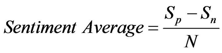 (1)
(1)
In addition, word frequency for each cluster’s tweets was calculated from each day’s data as a means of uncovering the primary topics discussed each day. Common stopwords such as pronouns and articles were removed from this word count to ensure meaningful words were most prominent. The list of stopwords to remove was taken from the stopwords corpus of the Natural Language Toolkit (http://nltk.org/). Once these procedures had been performed, it was easy to visualize changing sentiment for each cluster and for the dataset as a whole over the course of the 32 days in which data were collected.
3. Results
The community detection we performed with the Walktrap algorithm permitted sentiment analysis at three different levels: the entire @technet network, communities within the network, and topics referenced by a given community. At each level of granularity, the average sentiment was calculated for each day as described in Equation (1).
The Walktrap algorithm found 15 communities in the @technet network of various sizes. It was determined that community 3 was the most meaningful for comparison with the network as a whole as it was the largest detected community. Thus, this community was chosen for analysis. Furthermore, from the list of keywords calculated as described in section 2.3, three of the words tweeted most frequently (“http”, “microsoft”, and “windows”) were selected for further study.
3.1. Global Sentiment
The average sentiment in the @technet social network was positive every day, as shown in Figure 1. While the average varied by day, the variation was not significant relative to possible values, which are in the range of all real numbers. The low sentiment value was likely due to the predominately objective nature of tweets created by professionals in the @technet network.
3.2. Sentiment in Community 3
The sentiment average from community 3, shown in Figure 2, generally revealed a similar trend to the global sentiment. However, in community 3, sentiment scores varied over a wider range of values. Figure 2 also shows a local maximum after January 19th, whereas in the same period the global curve displays a local minimum. This is seen in the trend lines in the graphs. The greater sentiment variation in community 3 as compared to the global
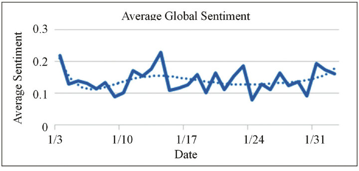
Figure 1. Average daily sentiment across all tweets in the @technet network. The solid line follows the sentiment data while the dotted line is a trend-line.
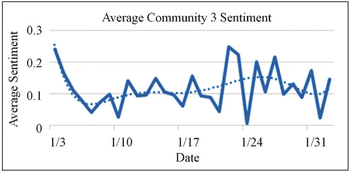
Figure 2. Average daily sentiment across all tweets in community 3 within the @technet network. The solid line follows the sentiment data while the dotted line is a trend-line.
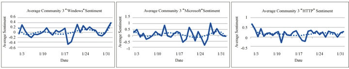
Figure 3. Average daily sentiment across all tweets for each of the keywords, “windows”, “http”, and “microsoft”, in the @technet network. The solid line follows the sentiment data while the dotted line is a trend-line.
network was driven by sentiment expressed towards specific topics. By examining the network at three levels (network, community, topic) we can investigate the way communities and topics within the @technet network affect the global sentiment trend.
3.3. Sentiment by Topic
Breaking down the sentiment results into multiple resolutions showed interesting trends, displayed in Figure 3. The average daily sentiment across community 3 between tweets containing the keywords “windows” and “http” demonstrated that sentiment associated with “windows” was more negative than for “http”. The topic “windows” also exhibited more fluctuation from day to day. The “http” curve shows similar variance, but this is less pronounced. Sentiment in tweets containing the word “microsoft” was trending upward during the first few days of data collection. This differs from the downward trend displayed for community 3 in Figure 2. The other interesting sentiment pattern was at day 23 when the overall slope was positive. This indicated positive community-level sentiment while “microsoft” was trending down, indicating conflicting opinions with the other two topics. The sentiment from all tweets created by community 3 and those containing the “microsoft” topic often reveal opposite trends. Furthermore, the sentiment curve for “microsoft” shown in Figure 3 demonstrates greater extremes than any of the other topics. It can be inferred from this that “microsoft” is a polarizing term.
3.4. Benefits of the Integrated Approach
The differences and similarities in sentiment observed at different levels of granularity reveal a greater amount of information about sentiment expressed within the @technet network. By combining sentiment analysis with community detection results, it becomes possible to easily view the sentiment expressed by different communities, comparing and contrasting this information with the network as a whole. This demonstrates the greatest benefit of integrating community detection and sentiment analysis; merging these two techniques permits more refined sentiment analysis.
4. Conclusion
Community detection and sentiment analysis are two important topics in the study of social networks. While these are generally treated as separate issues, this study adopted an integrative approach that enabled granular sentiment analysis on the level of individual communities. To do this, the Walktrap algorithm was used to detect communities on a network of Twitter users related to Microsoft Corporation’s @technet Twitter account. Sentiment analysis, facilitated by the SentiWordNet Lexicon, was then performed on the tweets created over 32 days by the communities in this network. Combining community detection output with sentiment analysis in this way permitted a more granular view of sentiment results. Comparing global sentiment from the @technet network with sentiment observed from a particular community regarding specific topics yielded more detailed information about sentiment expressed within this network. Thus, this study showed the sentiment information gained by merging community detection and sentiment analysis, demonstrating the value of integrating these two techniques.
5. Acknowledgements
We would like to thank Houghton College for its financial support.
REFERENCES
- S. Wasserman and K. Faust, “Social Network Analysis,” Cambridge University Press, Cambridgem, 1994. doi:10.1017/CBO9780511815478
- N. Gulbahce and S. Lehmann, “The Art of Community Detection,” BioEssays, Vol. 30, No. 10, 2008, pp. 934- 938.
- S. Fortunato, “Community Detection in Graphs,” Physics Reports, Vol. 486, No. 5-6, 2010, pp. 75-174. doi:10.1016/j.physrep.2009.11.002
- M. Girvan and M. Newman, “Community Structure in Social and Biological Networks,” Proceedings of the National Academy of Sciences, Vol. 99, No. 12, 2002, pp. 7821-7826. doi:10.1073/pnas.122653799
- M. Porter, J. Onnela and P. Mucha, “Communities in Networks,” Notices of the American Mathematical Society, Vol. 56, No. 9, 2009, pp. 1082-1097, 1164- 1166.
- H. Assael and J. Keon, “Nonsampling vs. Sampling Errors in Survey Research,” Journal of Marketing, Vol. 46, No. 2, 1982, p. 114.
- B. Liu, “Sentiment Analysis and Subjectivity,” Handbook of Natural Language Processing, 2nd Edition, CRC Press, New York, 2010.
- P. Bo and L. Lee, “Opinion Mining and Sentiment Analysis,” Foundations and Trends in Information Retrieval, Vol. 46, No. 1-2, 2008, pp. 1-135. doi:10.1561/1500000011
- B. O’Connor, R. Balasubramanyan, B. Routledge and N. Smith, “From Tweets to Polls: Linking Text Sentiment to Public Opinion Time Series,” Proceedings of the 4th International AAAI Conference on Weblogs and Social Media, Menlo Park, 2010, pp. 122-129.
- S. Tan and J. Zhang, “An Empirical Study of Sentiment Analysis for Chinese Documents,” Expert Systems with Applications, Vol. 34, No. 4, 2008, pp. 2633-2629. doi:10.1016/j.eswa.2007.05.028
- P. Pons and M. Latapy, “Computing Communities in Large Networks Using Random Walks,” Journal of Graph Algorithms and Applications, Vol. 10, No. 2, 2006, pp. 191-218. doi:10.7155/jgaa.00124
NOTES
*Corresponding author.