Communications and Network
Vol. 4 No. 2 (2012) , Article ID: 19094 , 10 pages DOI:10.4236/cn.2012.42014
Optimal Number of Relays in Cooperative Communication in Wireless Sensor Networks
Computer Science Department, Jordan University of Science and Technology, Irbid, Jordan
Email: {mardini,yaser}@just.edu.jo, saaleidi09@cit.just.edu.jo
Received November 30, 2011; revised January 25, 2012; accepted February 1, 2012
Keywords: Power Consumption; Wireless Sensor Networks; Optimal Number of Relays
ABSTRACT
Wireless Sensor Networks (WSN) typically consist of resource constrained micro sensors that organize itself into multihop wireless network. Sensors collect data and send it directly, or through intermediate hops in cooperative communication system, to the collection point. These sensors are powered up by batteries, for which the replacement or recharging is very difficult. With finite energy, we can transmit a finite amount of information. Therefore, minimizing the power consumption for data transmission becomes a most important design consideration for wireless sensor networks. In this paper, we discuss the optimal power consumption in cooperative wireless sensor network that are placed on a grid. We study different cases for the optimal power consumption in such grids by varying the grid distance and number of nodes in the grid. We assume the cases of grids from 2 × 2 up to 5 × 5 in increasing complexity of calculations. The results show that the optimal path that consumes the least power is the path along the diagonal using of the grid when the source and the destination and the furthest two nodes in the grid. This path takes intermediate nodes (relays) along it based on some threshold distances. For example, in 5 × 5 cases; the first threshold between the direct distance and between using one relay in the middle is 31.6 m the second threshold distance is 63.3 m after which using three relays is the best in power consumption between the source and the destination.
1. Introduction
Due to the tremendous growth in new and innovated wireless technologies that made it cheap and accessible, SN is steered toward wireless domain. Moreover, advancements in Global Positions System (GPS), cellular phones, and military applications, highlight the need for self-organized Wireless Sensor Networks (WSN) that can be characterized with optimal characteristics such as shortest route, lowest power consumption, and extended life time.
In addition, WSN has been introduced to lower the cost of connectivity to physical world compared with the wired alternative. The accuracy of the result and information obtained by such networks (WSNs) make them preferred by the researchers and the industry. This is due to their close proximity to physical phenomena, ease of deployment, low obtrusiveness and uniform coverage.
One of the important features of WSNs nodes is the power consumption since WSNs are usually deployed in remotely or inaccessible sites such as natural habitats, wild fires, and earthquake regions. This gives the need to find optimal routing paths and efficient power consumption algorithms for WSNs. WSN can be viewed as data acquisition network which is used to sense natural or man-made phenomena. It is critical to ensure that wireless sensor networks are capable of operating unattended for long durations. The lack of easy access to a continuous energy source in most scenarios and the limited lifetime of batteries have hindered the deployment of such network [1,2].
Power consumption is one of the important issues in wireless sensor networks. We note, a sensor node performs both computation and communication operation, a key observation is that communication operations consume considerable energy compared to computation operations. This observation can be further utilized to reduce power consumption.
WSN nodes connect together in an ad hoc fashion. However, due to the nature of their working environment and target applications, traditional routing algorithms for ad hoc networks fails to optimize the resource in WSNs [3]. Therefore, the need for new set of routing protocols specially designed for WSNs that considers power consumption more carefully [1,2,4].
Researchers tackled the main aspects of WSNs including routing efficiency [3], data aggregation [1], and group formation [2]. However, researchers conclude that for WSN, a more robust and worth trusty power consumption protocols are needed.
A node sensor is typically consists of memory that stores programs and intermediate data, a controller that processes either remove is or consisted of data and operate the other components, a limited energy supply (normally battery), transceiver that acts as a transmitter and receiver with a limited transmission range, and a sensor element that senses that ambient environment.
Sensor nodes collaborate to detect events or phenomena depending on the application. Each node collects a small amount of data and transmits it to the nearest sink node. This is done by hopping the data from node to node until it reaches the desired sink. Although the sensor nodes individually have limited capabilities, their collaboration to perform specific task produce an enhanced view of the physical world.
The limited capabilities of a single node make it alone undesirable to work or adopt but when deploying hundreds or even thousands of nodes, to work or monitor a phenomena, the overall and emerged benefits make it acceptable to overcome the limitation of a single node. Such emerging benefits are: data collection volume, fault tolerance, decrease cost, and accuracy enhancement.
Sensor nodes suffer many limitations, WSN require a mechanism to utilize the limited resources [5-7].
Energy Management Problems
The main challenge that might come into view when a group of nodes lose their energy is the developing of separate islands within the network. This will eventually leads to failure, or delay of the data collected. In WSN, such case is hard to manage manually as sensor nodes don’t consumed energy in a predicted approach [8].
Power consumption in sensor nodes can be classified into four categories: communication, sensing, inactive listening, and data processing. Comparing these feature shows that communication is a dominant feature in determining the rate of power consumption [7].
In addition to collecting data, sensor nodes are required to relay data for the other nodes. Therefore, nodes reside on the routing path are expected to have less energy than other neighboring nodes. If these nodes fail due to energy constrains, the network might be divided into several disconnected networks. Allowing the neighboring nodes to carry the burden of routing the data evenly will prevent this problem from appearing and hence increases the lifetime of the network [8].
Signal fading is defined as; how long the signal transmits before it reaches half its peak. This determines the radius of transmission for any antenna combined with the energy level that the antenna can bear. A node with more than one antenna will improve the transmission for that node but hence sensor nodes are limited with their energy, hardware and size, having one antenna is a constraint for such node.
Cooperative communication is introduced to solve such problem. This technique requires the collaboration of several nodes to act as one in terms of communication. A node that is sending a signal but has range and energy limitations might use other nodes antenna to achieve transmit variety. This process produces a variety of communication paths between the source and the destination nodes. By optimizing the intermediate nodes, an optimal relay path can be achieved.
The scope of this research is limited to exploring the problem of developing energy efficient communication approach in a grid topology with limited size and space. This paper will analyze the power consumption in grid topology to prolong the network lifetime by decreasing the power consumption in the overall grid. This can be done by optimizing the path from the source to the destination nodes.
This paper is divided into five sections as follows: Section 1 presents a brief introduction about wireless sensor networks and their properties, applications, challenges, energy management problem, and cooperative communication. Moreover, it highlights the main objectives of the study. Section 2 presents related work to energy efficiency in wireless sensor network. Section 3 introduces the network models. Section 4 presents detailed description of the simulation environment and the obtained results. Finally Section 5 concludes the paper and presents some challenges and open questions for the future work.
2. Related Work
A wireless sensor network is a collection of nodes with limited energy and computation engine that work together to construct a network that monitor a certain phenomena [3]. The study presented in [1] emphases on power consumption as the crucial factor for surviving when talking about WSNs. Data processing normally goes through a certain layers that can be implemented with sufficient intelligence towards power consumption [2].
Aksu and Ercetin [4] stated that to improve transmission diversity for some WSNs, nodes should have more than one antenna but due to energy, hardware and size limitations, that requirement is almost impossible to achieve. Cooperative communication is introduced to overcome such challenge by allowing a couple of nodes to share their antenna to achieve a multiple-antenna (virtually more than one antenna for each node).
In [5], low data rates and power consumption is traded off according to the distance from source to distention to achieve the best schema for Power consumption. The most relevant work have been carried on by [9], the authors proposed tradeoff in cooperative system that require low transmission energy than another system under Bit Error Rate (BER) performance measure, while allowing sensor nodes to cooperate and exchange local data before transmission.
Muhammad and Md. Abdual [10] proposed a new hierarchical routing protocol for efficient energy to increase the lifetime of cluster based wireless sensor networks and eliminates overhead of dynamic cluster in LEACH and PEGASIS protocols which form chain among the nodes so that each node will receive from and send to close neighbor. Chen and Kuo [11] study routing for wireless sensor networks that are based on grid topology. They used transmission cost to analyze the distance between the nodes in the grid. Based on the obtained results, the authors proposed a new cost parameter, defined as metric, to selected nodes in the grid by considering the remaining the power and location of relays and used this cost parameters to select forwarding path.
Akl and Sawant [12] find the grid size based on coordinate routing algorithm in wireless sensor network, the authors compare the power consumption in wireless sensor networks for different grid sizes. In their work, the source node floods to all coordinator in the network, where the coordinators are elected in the grid.
Dhanapala and Han [13] proposed a method of evaluating the probability of sending packet within a number of hops in random routing protocol to determine the right neighbor to send data to in the grid. They also, derive probability for packet sending within the nodes as well as the convergence probability of agent and queries with number of hops. Authors in [14] studied the effect of three performance metrics: coverage, message transmitting delays, and power consumption in sending and receiving data in nodes, on the random and deterministic sensor deployment for large area wireless sensor networks. It considers three topologies: a square grid, a uniform random and a pattern based Tri-Hexagon tiling sensor nodes models.
In [15], the authors used a hybrid of data and decision fusion algorithms to understand the relationship between network coverage and power consumption for enhanced sensing range in cooperation system when sensors exchange data. The authors take into account the possible applications in wireless sensor network to extend the network’s life time while maintaining constrains on false alarm and missing probability. Elhawary and Haas [16] proposed a new protocol to enable cooperative system transmission between sending cluster nodes and receiving cluster nodes to minimize the power consumption in communication packets and increase transmission reliability. In [17], Le and Hossain proposed two distribution algorithms based on two layer optimization frameworks for cooperative wireless sensor networks using diversity gain from cooperative communication.
In [18], Chen et al. obtained diversity gain and energy saving to enhance the network lifetime using cooperative data transmission scheme for cluster heads in wireless sensor network that are based on grid cluster model. Yu et al. [19] proposed a new cluster routing protocol for wireless sensor network based on grid topology to provide an energy efficient schema.
The work in [20] shows a study of the effect of cluster size over the power consumption in cooperative wireless sensor networks. When the wireless sensor networks are separated into a number of clusters, any sensor node in every cluster will send the data to sink node. They proposed optimal sectoring for the network using cooperative sensors to reduce the power consumption. Tan in [21] design an algorithm to minimize the power consumption in wireless sensor networks. The algorithm, he studied two issues: using of a scheduling algorithm to separate the entire sensor nodes into different grid groups. While the other was using priority rules to decide which of sensor should be on and which should be off in an active duration time.
Ahmed et al. [22] divided the wireless sensor network into two functional models within the link layer. The first model is deals with linking all the sensor nodes in network—except the sensor nodes in backbone link that are near base station—with Ricean fading channel. For the excepted sensors that are near the sink, they are grouped via a link model with pure deterministic channel. The author in [23] extends the Two-Tier Data Dissemination (TTDD) protocol to create virtual grids within the network to reduce the number of relays needed to forward the data to the destination. However, that didn’t solve the problem of hot spots in the network.
The work in [24] is another extends the TTDD protocol but it employs the XY geographical routing to forward the packets using the grid-based architecture having fixed sensor nodes responsible for data relaying. It has the same problem of unpredicted battery discharge because the nodes responsible for data sending are fixed.
Rajendran et al. Reference [25] Reduce the probability of packet loss that happens with the collision and transmitting in sleep mode. They presented new protocol to extend the life time on wireless sensor network lifetime. The traffic-adaptive medium access protocol (TRAMA) which is a new protocol with energy-aware channel accesses for sensor nodes in networks. In [26], the authors proposed a scenario to study the factors which would increase the number of relays in multi hop wireless sensor networks for power consumption. We consider the maximum data rate and study the effect of the distance in the linear and random paths for the power consumption to achieve the optimal number of relays to deliver the packets.
Authors in [27] proposed new greedy protocol that is an improvement over LEACH protocol. Power Efficient Gathering in Sensor Information System (PEGASIS) protocol increases the life time and quality of the wireless sensor networks. It eliminates the overhead of cluster construction and limits the number of send and receives operations among all the sensor nodes using one node to forward the information to the base station per round. In this work, the authors used first order radio model where the radio dissipates Eelec = 50 nJ/bit for both the transmitter and receiver circuitry and Єamp = 100 pJ/bit for the transmission amplifier.
In [28], the authors presented two approaches to transmit the collect data from sensor nodes to the base station, the first one is direct approach, and it sends data directly to the base station which located far away from the node. Therefore, the direct transmission will consume large amount of transmission power from sensor nodes and this will quickly consume the nodes’ battery and reduce the network life time. To utilize the energy, a second approach was proposed, called LEACH protocol, which is designed to organize the sensors into clusters with one sensor is elected as cluster head to aggregated and transmit the data to the base station.
Reference [29] presented a new approach for energy aware routing in wireless sensor networks where sensor nodes and base station are assumed to be mobile. Sensor system for Hierarchical Information gathering through Virtual triangular Areas (SHIVA) is proposed to observe energy efficiency and consider a hierarchical deployment of the network and consider a rectangular 2-dimensional sensor field.
3. Methodology and Network Model
As mentioned earlier power consumption is critical for sensor networks. Sensor nodes consume battery energy to transmit the data from node to another. The amount of the power consumption depends on the distance between the transmitter and the receiver nodes, and the amount of data transmitted. There are two modes of operations for sensor nodes: Fixed and adaptive energy levels. In this paper, we assume that the nodes use the adaptive energy mode. We next present the mathematical analysis for various grid topologies.
3.1. Energy Analysis in Wireless Transmission
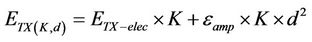
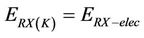
The source node can send the data to the destination node using one or more relay nodes, rather than directly, to reduce the power consumption. Each relay node acts as a router that forwards the received packets from one neighbor to another. The relay node consumes three kinds on energy when forwarding the packet; energy to receive the data, energy to amplify the data signals and energy to transmit the data. This can be expressed using (1) and (2) as follows [5]:
 (1)
(1)
 (2)
(2)
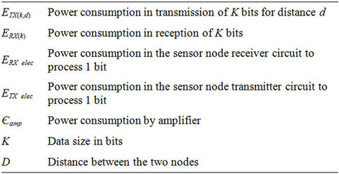
where:
Note that the amplified energy is increased in the square of the distance. Thus, reducing the power consumption by introducing more relays will have a great effect to reduce the power consumption to amplify signals since the sum of the square distance of segments are much less that the square distance of the total distance. In other words, if d = d1 + d2 +∙∙∙dh then 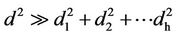 . However, at each relay, there is extra energy needed to receive and retransmit the data. Thus, it is a tradeoff to balance between these two types of reduction and increment in power consumption to achieve optimal total value.
3.2. Network Model
The 2-D grid topology is considered in this paper. In this topology, nodes are aligned in a 2-D grid, and the nodes are fixed and equally spaced from each other [11]. We consider a network topology that consists of a 2-D grid with total number of nodes equal to N × N, where N is the total number of nodes in a row/column. drow represents the distance from the first node to the last node in the same row/column.
Moreover, we assume all nodes; initially have the same energy level. Relays are responsible for forwarding the packet it receives from other nodes or relays. In such topology, the distance between two adjacent nodes is (drow/(N – 1)). This topology is depicted in Figure 1.
4. Analysis and Experimental Results
4.1. Energy Analysis in Grid Network
Without loss of generality, power consumption analysis is done for 1-bit message sent from the source to the destination nodes in grid topology. When using relays, the total power consumption between the source and destination will be:
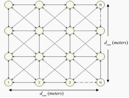
Figure 1. N × N grid topology.
 (3)
(3)
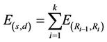
where,  is the power consumption to send the data from node Ri–1 to node Ri. R0 is the source node and Rk is the destination node. K is the number of nodes in the path from the source to the destination.
In the following cases, we assume that the source and the destination nodes are the farthest two nodes in the grid. Our analysis will be inductive by showing the results for 2 × 2, 3 × 3, 4 × 4, and 5 × 5 grids. Before we proceed with the analysis, we introduce the parameters used in the experimental results presented at each case later on.
4.2. Analysis and Experimental Results for 2 × 2 Grid
In 2 × 2 grid, the source node 1 can send data to the destination node 4 via various possible paths. The source node 1 sends the data to via its neighbor node 2 or node 3, then this node forward the data to the destination node 4. Another possible path, the source node can send the data directly to the destination node. Moreover, node 1 can send data to node 2, then node 2 sends data to node 3, and finally node 3 sends data to node 4. This path is clearly not optimal with respect to the power consumption.
Note that the distance from node 1 to node 2 is the same as the distance from node 2 to 4 and equals , while the direct distance (diagonal) is
 .
.
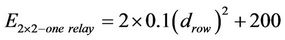
So if the data is sent via node 2 or 3 then the power consumption after applying (1) and (2) and by using Єamp = 100 pJ/bit/m2, ERX_elec = 50 nJ/bit, ETX_elec = 50 nJ/bit [10,26,29].
 (4)
(4)
If the direct transmission is used, then the power consumption is:
 (5)
(5)
So both (4) and (5) simplifies to same values expect constant term (100 or 200). Thus, using one relay will always have more power by 100 units than the direct transmission.
Figure 2 presents the relationship between power consumption in the direct path (diagonal) grid and another path (one relay) alternative for various drow values in 2 × 2 grid.
4.3. Analysis and Experimental Results for 3 × 3 Grid
In the case of 3 × 3 grid, we assume case that the source node 1 sends the data to the destination node 9. We consider various possible paths. First, the source node can send the data directly to the destination. Or it can sends the data via its neighbor nodes 2, 4 or 5, and then these nodes can forward the data via its neighbors to the destination node 9.
Figure 3 presents power consumption for the two options of the diagonal paths: direct and one relay. As we explained before, using the diagonal direction the source can send the data to the destination with two possible options; directly or using one relay at the middle.
The distance from the source to the destination in one relay equals:
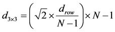 (6)
(6)
The total energy needed for direct transmission in (1) and (2) and by using Єamp= 100 pJ/bit/m2, ERX_elec =50 nJ/bit, ETX_elec =50 nJ/bit [10,26,29].
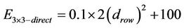 (7)
(7)
For one relay path, the power consumption is given in (8):
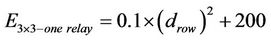 (8)
(8)
In this type of network 3 × 3 grid topology can be concluded the following.
Lemma 1:
Threshold distance when transmission via the direct path (diagonal) between the source and the destination nodes, similar the transmission using one relays is:
Proof:
Set (7) to be equal (8) implies:
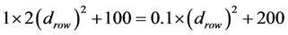
Implies

Therefore, when the distance less than 31.6 m, direct
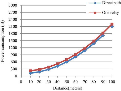
Figure 2. Power consumption in 2 × 2 grid.
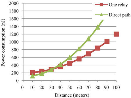
Figure 3. Power consumption in two cases in diameter 3 × 3 grid.
transmission is better than using one relay paths in 3 × 3 grid, while one relay is better for distances more than 31.6 m.
4.4. Analysis and Experimental Results for 4 × 4 Grid
As shown previously, the diagonal path is the optimal path in the grid. Therefore, this paper consider comparing the following three paths only: in the first path, the source node transmit to the destination node directly without using any relay nodes, in this case, the direct diagonal distance equal . The second path uses one relay in the diagonal to deliver data to the destination node; this can be either the node 6 or 11, and then the data is sent to the destination node 16 directly. In the third option, two relay are used, the data is first sent to node 6 then to node 11 and finally to the destination node. The distance between nodes 1 and 6 equals
 .
.
Therefore, we apply (1) and (2) to find power consumption for the direct transmission:
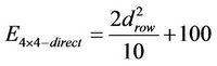 (9)
(9)
For one relay path, the power consumption is given in (10):
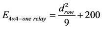 (10)
(10)
For two relays path, the power consumption is given in (11):
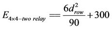 (11)
(11)
It is clear from our previous results that direct transmission would be optimal up to certain point, then using one relay would be enough and after a certain threshold two relays would be better.
Lemma 2:
Threshold distance between the optimal power consumption using direct transmission and using one relay in 4 × 4 grid is 33.54 m.
Proof:
Set (9) and (10) together to get:
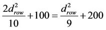
Implies
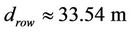
Lemma 3:
Threshold distance between the optimal power consumption using one relay and using two relay in 4 × 4 grid is 47.4 m.
Proof:
Set (10) and (11) together to get:
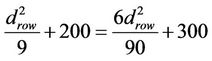
Implies
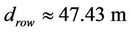
Figure 4 explains lemma 3, using threshold distance in 3 × 3 grid is 31.6 m to find threshold distance in 4 × 4. As show previously threshold distance in 4 × 4 equal 47.43 m Therefore, when the distance less than 47.43 m the source node transmits directly through the 3 × 3 grid to the distention node but when the distance more than 47.43 m the source transmits through one relay in 3 × 3 grid.
Figure 5 depict some numerical results for Equations (11), (12) and (13).
4.5. Analysis and Experimental Results for 5 × 5 Grid
In this case, sensor nodes are deployed in 5 × 5 grid
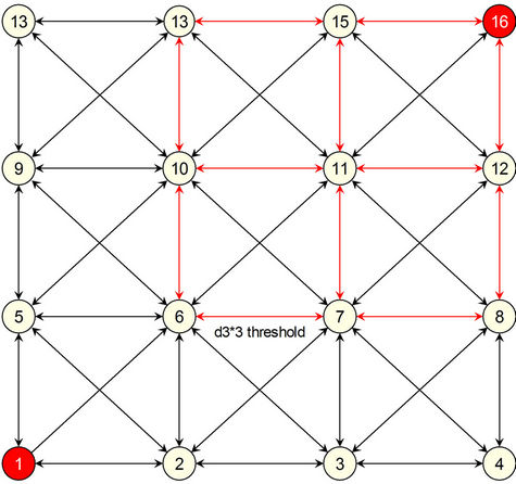
Figure 4. Threshold distance in 4 × 4 grid.
Figure 5. Power consumption in three cases in diameter 4 × 4 grid.
where the source and the destination node are the farthest two nodes in the network. Similar cases can be studied along the diagonal to transmit using no relay, one, two, or three relays.
The power consumptions for the cases mentioned above are:
Direct path:
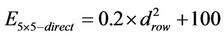 (12)
(12)
One relay (case 1): (node 13) in the middle of the diagonal:
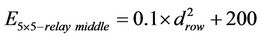 (13)
(13)
One relay (case 2): (node 7) located in the distance closest to the source node or one relay (node 19) located in the distance closest to the destination node will have the same result:
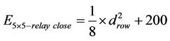 (14)
(14)
Two relays: we have three cases:
• Two relays (node 7 and 13) at the source side.
• Two relays (node 13 and 19) at the destination side.
• Two relays (node 7 and 19); one near the source and one near the destination.
Each case has the same power consumption because each case has two short transmissions (one block in the grid) and one large transmission (two blocks in the grid)
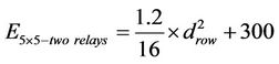 (15)
(15)
Three relays: (nodes 7, 13 and 19):
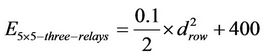 (16)
(16)
For the case of 5 × 5 grid, we will have the following three lemmas.
Lemma 4:
Threshold distance between the optimal power consumption using direct path and using one relay in 5 × 5 grid is 31.6 m.
Proof:
Set (12) and (13) together to get:
Implies
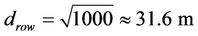
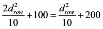
Lemma 5:
Threshold distance between the optimal power consumption using one relay path and using two relays in 5 × 5 grid is 63.3 m.
Proof:
Set (13) and (15) together to get:
Implies
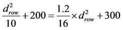
Lemma 6:
Threshold distance between the optimal power consumption using two relay paths and using three relays in 5×5 grid is 36.3 m.
Proof:
Set (15) and (16) together to get
Implies
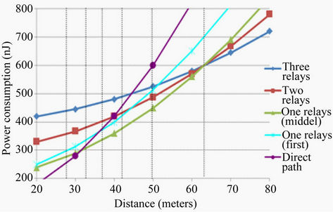
Figure 6 presents the relationship between the power
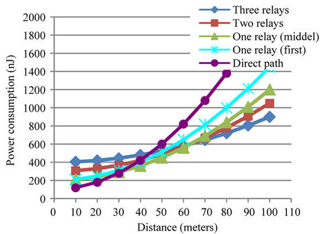
Figure 6. Power consumption in five cases in diameter 5 × 5 grid.
consumption for different paths along the diagonal and various distances for drow in 5 × 5 grid. In summary, the direct transmission is the best up to 31.62 m, and then using one relay would give optimal power consumption up to distance 63.3 m. After that, three relays will be the choice. Figure 7 shows zooming for the intersection points of Figure 6. Moreover, in 2 × 2 grid the direct path is optimal regardless the grid distance. In 3 × 3 cases, the diagonal option is the optimal without relays in the middle for distances from 10 m to 30 m, however, the diagonal option with one relay is optimal for distances greater than 31.6 m.
In the 4 × 4 cases, the results shows that the diagonal option is the optimal without relays if the distance is less than 30 m, however, the diagonal option with one relay is optimal for larger distance than 33.54 m. Another intersection point is between the one relay and two relay options at 47.43 m and the two relay is optimal when the distance increase up to 47.43 m. In the 5 × 5 cases, the direct transmission is the optimal up to 31.62 m, and the optimal for one relay is at distance 63.3 m. After that, three relays is the optimal path.
By comparing the results of 3 × 3 grid and 5 × 5 grid, we note that the common node of 31.6 m appeared in the threshold distances. Note that this can be justified since 5 × 5 can be divided into two 3 × 3 grids with one node in common, so the optimal for the cases of 3 × 3 can be added up with the node in the middle.
5. Discussion
The directcommunication scheme has the worst performance because the source node consumes more energy to transmit data directly to the destination node. But this is different when using multi-relays between the sources and the destination nodes, to saving the power consumption toextend network lifetime.
The simplest routing algorithms are the flooding algo-
rithms in which each node retransmits any packet that it receives over the network.
Figure 8 represent optimal power consumption in different constant distance, to transmit the data between the source and the destination nodes. Where the power consumption increases when the distance increases.
Figure 9 represents optimal number of relays in fixed distance with different grids size; this figure shows the result obtained that when the distance is less than 30 m, then sending directly to the destination node via the optimal path. Moreover, results present that using one relay node to reduce the power consumption when the distance between 40 m to 50 m, and the optimal number of relays increasing when the distance increase.
Figure 10 shows the relationship between the grid size and the power consumption where I took about one cases when the distance 90 m, where the power consumption is minimum when the number of relays nodes equal three relays with 5 × 5 grid.
6. Conclusions and Future Work
Wireless sensor networks are an emerging area with the potential of many applications that varies from military to civilian domains. Power consumption is the key challenge that faces the deployment of WSNs as the network consists of small nodes with limited processing, storage, communication, and energy capabilities. Several deployment methodologies exist for deploying the nodes. Nodes can be spread randomly or in a grid topology. Deployment strategy depends on several factors such as type of application physical limitation, and the optimal usage of nodes scare energy.
In this paper we focus our attention on the 2-D grid topology and investigate the optimal path (i.e. number of relays) for power consumption. Several thresholds for distance exist for the optimal path. Direct transmission is the optimal path for close the nodes (i.e. short distance. As the distance increase, number of relays increase).
For future work, we propose to future investigation the
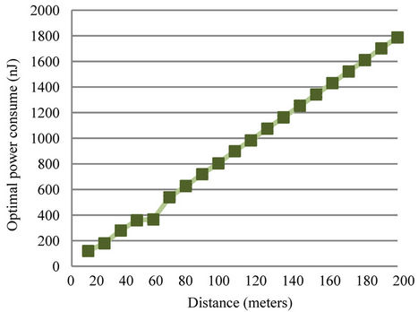
Figure 8. Power consumption with fixed distance grid.
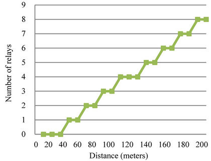
Figure 9. Optimal number of relays with fixed grid.
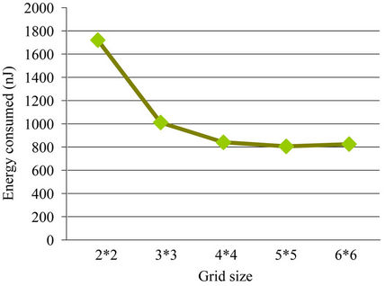
Figure 10. Power consumption in different grid size with distance 90 m.
power consumption issue for other topologies such as random deployment of the sensors. Moreover, numerical and theoretical results need to be obtained for network of large sizes. The conclusion drawn by numerical experiment and mathematical modeling in this paper can be further utilized to design a power-efficient routing protocol for WSNs. The proposed protocol strives to select the optimal path all time. In this paper, we define optimality in terms of power consumption only. It might be worthwhile to express define optimality in terms of other performance metrics such as data rate and diversity gain in addition to power consumption.
REFERENCES
- V. Raghunathan, C. Schurgers, S. Park and Srivastava MA, “Energy-aware Wireless Microsensor Network,” Signal Processing Magazine, Vol. 19, No. 2, 2002, pp. 40-50. doi:10.1109/79.985679
- K. Romer and F. Mattern, “The Design Space of Wireless Sensor Networks,” Wireless Communications, Vol. 11, No. 6, 2004, pp. 54-61.
- W. Ye, J. Heidemann and E. Estrin, “An Energy-Efficient MAC Protocol for Wireless Sensor Network,” Proceedings of the 21st Annual Joint Conference of the IEEE Computer and Communications Societies, New York, 23- 27 June 2002, pp. 1567-1576.
- J. Yick, B. Mukherjee and D. Ghosal, “Wireless Sensor Network Survey,” Computer Networks: The International Journal of Computer and Telecommunications Networking, Vol. 52, No. 12, 2008, pp. 2292-2330. doi:10.1016/j.comnet.2008.04.002
- I. Joe and S. Chung, “The Distance-Power Consumption Tradeoff for Cooperative Wireless Sensor Networks,” Communications in Computer and Information Science, Vol. 56, 2009, pp. 180-187. doi:10.1007/978-3-642-10844-0_23
- C. Chong and S. Kumar, “Sensor Networks: Evolution, Opportunities, and Challenges,” Proceedings of the IEEE, Vol. 91, No. 8, 2003, pp. 1247-1256. doi:10.1109/JPROC.2003.814918
- K. Islam, “Energy Aware Techniques for Certain Problems in wireless Sensor Networks,” Ph.D. Thesis, QUEEN’S University, Kingston, 2010.
- C. Alippi, G. Anastasi, M. Francesco and M. Roveri, “Energy Management in Wireless Sensor Networks with Energy-Hungry Sensors,” IEEE Instrumentation and measurement Magazine, Vol. 12, No. 2, 2009, pp. 16-23. doi:0.1109/MIM.2009.4811133
- Y. Gai, L. Zahng and X. Shan, “Energy efficiency of Cooperative MIMO with Data Aggregation in Wireless Sensor Networks,” IEEE Wireless Communications and Networking Conference, Kowloon, 11-15 March 2007, pp. 11-15. doi:10.1109/WCNC.2007.151
- M. Hussain and M. Mottalib, “Energy-Efficient Hierarchical Routing Protocol for Homogeneous Wireless Sensor Network,” IJCSNS International Journal of Computer Science and Network Security, Vol. 1, No. 1, 2011, pp. 80-86. doi:10.1109/ICMCS.2011.5945618
- Y. Chen and C. Kuo, “Integrated Design of Grid-Based Routing In Wireless Sensor Networks,” Proceedings of the 21st International Conference on Advanced Information Networking and Applications (AINA), Niagara Falls, 21-23 May 2007, pp. 625-631.
- R. Akl and U. Sawant, “Grid-based Coordinated Routing in Wireless Sensor Network,” Proceedings of the 4th IEEE Consumer Communications and Networking Conference, Las Vegas, 11-13 January 2007, pp. 860-864. doi:10.1109/CCNC.2007.174
- D. Dhanapala, A. Jayasumana and Q. Han, “Performance of Random Routing on Grid-Based Sensor Networks,” Proceedings of the 6th IEEE Consumer Communications and Networking Conference, Las Vegas, 10-13 January 2009, pp. 1-5.
- W. Poe and J. Schmitt, “Node Deployment in Large Wireless Sensor Networks: Coverage, Power Consumption, and Worst-Case Delay,” Proceedings of the 5th ACM SIGCOMM Asian Internet Engineering, Bangkok, 10-13 January 2009, pp. 978-981.
- W. Wang, V. Inivasan, K. Chua and B. Wang, “EnergyEfficient Coverage for Target Detection in Wireless Sensor Networks,” Proceedings of the 6th international conference, Cambridge, 25-27 April 2007, pp. 313-322.
- M. Elhawary and Z. Haas, “Energy-Efficient Protocol for Cooperative Networks,” IEEE/ACM Transaction on Networking, Vol. 19, No. 2, 2011, pp. 561-574. doi:10.1109/TNET.2010.2089803
- L. Le and E. Hossain, “Cross-layer Optimization Frameworks for Multihop Wireless Networks Using Cooperative Diversity,” IEEE Transactions on Wireless Communications, Vol. 7, No. 7, 2008, pp. 2592-2602. doi:10.1109/TWC.2008.060962
- X. Chen, C. Pan, Y. Zhou and Y. Cai, “Cooperative Data Transmission Utilizing Neighboring Cluster Head Over WSNS,” International Symposium on Intelligent Signal Processing and Communication Systems, Vol. 4, 2007, pp. 432-434. doi:10.1109/ISPACS.2007.4445916
- L. Y. Yu, W. Zhang and C. Zheng, “GROUP: A GridClustering Routing Protocol for Wireless Sensor Networks,” International Conference on Wireless Communications, Networking and Mobile Computing, Wuhan, 22-24 September 2006, pp. 22-24. doi:10.1109/WiCOM.2006.287
- H. Sarma, A. Kar and R. Mall, “Energy Efficient Communication Protocol for a Mobile Wireless Sensor Network System,” International Journal of Computer Science and Network Security, Vol. 9, No. 1, 2009, pp. 386- 394. doi:10.1109/HICSS.2000.926982
- H. Tan, “Maximizing Network Lifetime in Energy-Constrained Wireless Sensor Network,” Proceedings of the International Conference on Wireless Communications and Mobile Computing, Vancouver, 3-6 July 2006, pp. 10876-10895.
- I. Ahmad, M. Peng and W. Wang, “Exploiting Geometric Advantages of Cooperative Communications for Energy Efficient Wireless Sensor Networks,” International Journal of Communications, Network and System Sciences, Vol. 1, No. 2, 2008, pp. 55-61. doi:10.4236/ijcns.2008.11008
- H. Luo, F. Ye, J. Cheng, S. Lu and L. Zhang, “TTDD: Two-Tier Data Dissemination in Large-Scale Wireless Sensor Networks,” Wireless Networks, Vol. 11, No. 1, 2005, pp. 161-175. doi:10.1007/s11276-004-4753-x
- M. Jin, Y. Choi, F. Yu, E. Lee, S. Park and S. Kim, “A Energy Efficient Data-Dissemination Protocol with Multiple Virtual Grid in Wireless-Sensor Network,” Proceedings of the Asia-Pacific Conference on Communications, Bangkok, 18-20 October 2007, pp. 377-380.
- V. Rajendran, K. Obraczka and J. Aceves, “Energy-EffiCient, Collision-Free Medium Access Control for Wireless Sensor Networks,” Proceedings of the 1st International Conference on Embedded Networked Sensor Systems, Los Angeles, 5-7 November 2003, pp. 419-438.
- W. Mardini, Y. Khamayseh and M. Salayma, “Optimal Power Consumption in Cooperative WSNs for a Random Distance Using a Linear Propagation Model,” The 2nd International Conference on Ambient Systems, Networks and Technologies, Niagara falls, 19-21 September 2011, pp. 489-496.
- P. Balamurugan and K. Duraiswamy, “Chain Based Energy Proficient Data Gathering Protocol for Wireless Sensor Networks,” International Journal of Computer Science and Technology, Vol. 2, No. 3, 2011, pp. 95-99.
- W. Heinzelman, A. Chandrakasan and H. Balakrishnan, “Energy Efficient Communication Protocol for Wireless Microsensor Networks,” Proceedings of the 33rd Annual Hawaii International Conference on System Sciences, Washington DC, 4-7 January 2000, pp. 1-10.
- H. Red, B. Abolhassani and M. Abdizadeh, “Lifetime Optimization via Network Sectoring in Cooperative Wireless Sensor Networks,” Networking and Communications, Vol. 2, No. 2, 2010, pp. 905-909. doi:10.4236/wsn.2010.212108