Received 16 February 2015; accepted 7 December 2015; published 10 December 2015

ABSTRACT

The Weber-Hermite differential equation, obtained as the dimensionless form of the stationary Schroedinger equation for a linear harmonic oscillator in quantum mechanics, has been expressed in a generalized form through introduction of a constant conjugation parameter according to the transformation, where the conjugation parameter is set to unity () at the end of the evaluations. Factorization in normal order form yields -dependent composite eigenfunctions, Hermite polynomials and corresponding positive eigenvalues, while factorization in the anti-normal order form yields the partner composite anti-eigenfunctions, anti-Hermite polynomials and negative eigenvalues. The two sets of solutions are related by an -sign reversal conjugation rule. Setting provides the standard Hermite polynomials and their partner anti- Hermite polynomials. The anti-Hermite polynomials satisfy a new differential equation, which is interpreted as the conjugate of the standard Hermite differential equation.

Keywords:

Weber-Hermite Differential Equation, Eigenfunctions, Anti-Eigenfunctions, Hermite, Anti-Hermite, Positive-Negative Eigenvalues

1. Introduction

The Weber-Hermite differential equation arises as the dimensionless form of the one-dimensional stationary Schroedinger equation for a linear harmonic oscillator of mass m, angular frequency, total energy E and displacement x obtained in quantum mechanics in the form [1] - [4] ,

. (1a)

Introducing parameters s and defined by

(1b)

we easily transform Equation (1a) into the dimensionless form

(1c)

which we call the Weber-Hermite differential equation, since its general solutions are the Weber-Hermite func- tions composed of the Hermite polynomials [1] - [4] .

It is convenient to replace

(1d)

to express Equation (1c) in the familiar mathematical form

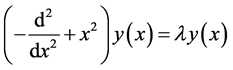. (1e)

We provide conjugate pairs of solutions of this equation through factorization.

We define a conjugation parameter and develop the factorization procedure in Section 2. Normal-order solutions in terms of composite Hermite polynomials, their recurrence relations, positive eigenvalues and differential equation are presented in Section 3.1, while the composite anti-Hermite polynomials, their recurrence relations, negative eigenvalues and differential equation arising from the anti-normal order solutions are contained in Section 3.2.

Factorization and the Conjugation Parameter

Factorization is a powerful technique for solving second-order ordinary differential equations. An important feature of factorization is factor ordering in the resulting product of factors, especially if the factors are operators [1] . To take account of operator factor ordering in general form, we introduce a constant parameter, which is set to unity () at the end of the evaluations, according to a transformation rule

(2a)

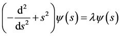
to express the Weber-Hermite Equation (1e) in the general form

(2b)

which is the same as Equation (1e) for.

Even though the main motivation for introducing the parameter is to account for operator ordering, it turns out that plays a fundamental role as a conjugation parameter, which provides a conjugation rule relating the two alternate normal and anti-normal order factorized forms of Equation (2b). The general solutions of the nor- mal or anti-normal order forms are conjugate polynomials related by the -conjugation rule.

Noting that the operator takes the form of a difference of two squares, we apply an effective factorization procedure [1] to express Equation (2b) in two alternately ordered forms

(3a)

(3b)

The operators are related by -sign reversal conjugation rule

(3c)

giving

(3d)

The operators are said to be -sign reversal conjugates satisfying conjugation rule (3c) according to notation

(3e)

where we have adopted the usual Hermitian conjugation notation using the symbol to apply in general. For operators or eigenfunctions expressible in matrix form, the Hermitian conjugation under the -sign reversal conjugation is effected by applying the conjugation rule (3c) to every element and then taking the transpose.

We note that in a case where, which would arise from an equivalent mathematical operation

(3f)

the -conjugation would constitute the familiar Hermitian conjugation rule, which justifies the use of the Her-

mitian conjugation notation adopted here. We observe that the mathematical operation in Equation (3f) applies to the factorization of a second order operator of the form.

According to the conjugation rule in Equation (3c), the factorized forms (3a) and (3b) are -sign reversal conjugates. Subtracting Equation (3a) from Equation (3b), using the conjugation relation (3e) and dropping the arbitrary function, we obtain the commutation relation

. (3g)

For reasons which may become clear below, we recognize as a lowering operator and

as a raising operator. In this respect, the factorized form (3a) is said to be in normal order, while the form (3b) is in anti-normal order.

2. General Solution

Since Equations (3a) and (3b) are related by the -conjugation rule (3c), their general solutions are -sign reversal conjugates. The normal order form (3a) yields the standard eigenfunctions, Hermite polynomials and the corresponding positive eigenvalues, while the anti-normal order form (3b) yields anti-eigenfunctions, anti-Hermite polynomials and the corresponding negative eigenvalues.

2.1. Normal-Order Form: Eigenfunctions, Hermite Polynomials and Positive Eigenvalues

We start by considering that the normal order form (3a) is an eigenvalue equation with eigenvalue. It has a lower bound of zero eigenvalue obtained as

(4a)

where denotes the lowest value of obtained at zero eigenvalue. The corresponding lowest order eigen- function at zero eigenvalue () is determined through Equation (3a) under the condition (4a) according to

. (4b)

Applying Hermitian conjugation of the operators and according to Equation (3e), we express Equation (4b) in the form

(4c)

which on multiplying from the left by the ε-sign reversal conjugate of the lowest order eigenfunction takes the form

. (4d)

The basic equation for the lowest order eigenfunction then follows from Equation (4d) in the form

(5a)

with a simple solution

(5b)

noting that the integration constant evaluated at is.

Eigenfunctions of general order are generated through repeated application of the conjugate operator

on the lowest order eigenfunction according to

(5c)

which on substituting from Equation (5b) and evaluating for give the first two lower order eigenfunctions in the form

. (5d)

To evaluate higher order eigenfunctions, , we derive a simplifying formula for any functions, in the form

(5e)

and then apply the general relation

(5f)

which follows easily from Equation (5c) by setting.

For, Equation (5f) gives

(6a)

which on substituting from Equation (5d) and applying the formula (5e) with, , then using Equation (5f) in the final step gives

. (6b)

Proceeding in the same manner for

(6c)

easily gives the forms

. (6d)

We arrive at the important general result that higher order eigenfunctions are obtained in the form of a re- currence relation

. (6e)

Setting in Equation (6e) and substituting lower order eigenfunctions as appropriate, recalling from Equation (5b) or (5d), we obtain the general eigenfunction in the form

(7a)

where is a polynomial depending explicitly on the parameter. For reasons which will be clear below, we shall call the composite Hermite polynomials, the general eigenfunctions are called the composite Weber-Hermite functions.

Using Equation (5b) in Equation (5c) and substituting the result on the l.h.s. of Equation (7a) provides the general relation for generating the composite Hermite polynomials in the form

. (7b)

Using Equation (5b) together with its -sign reversal conjugate

(7c)

in Equation (7b) defines the composite Hermite polynomials in terms of the lowest order eigenfunction accord- ing to

. (7d)

Explicit forms of are easily obtained using a recurrence relation derived in the next subsection.

2.1.1. Recurrence Relations and Differential Equation for

Setting in Equation (7b) and inserting as appropriate, then using Equation (7b) gives the relation

(8a)

which is easily evaluated to obtain the first recurrence relation for the polynomials in the form

. (8b)

Setting in Equation (7b) gives

. (8c)

Setting in Equation (8b) then provides the first five composite Hermite polynomials as

(8d)

taking the general expansion

. (8e)

The symbol in the summation means that m runs over integer values up to the integer part of, e.g.,

,. The general form in Equation (8e) clearly displays the explicit dependence of the polynomials on the parameter, which provides the justification for calling the composite Hermite polynomials, since the polynomials become the standard Hermite polynomials after setting, while setting transforms the polynomials to their conjugation partners.

Substituting

into Equation (6e) gives the second recurrence relation for the composite Hermite polynomials in the form

. (8f)

Comparing the first recurrence relation (8b) and the second recurrence relation (8f) easily provides the third recurrence relation for the composite Hermite polynomials in the form

. (8g)

Applying on Equation (8g) gives

. (9a)

Using Equation (8e) together with the result of setting in Equation (8g) gives

(9b)

which we substitute into Equation (9a) to obtain the differential equation for the composite Hermite polynomials in the form

(9c)

which differs from the familiar Hermite differential equation [1] - [10] only by the factor on the second order derivative term. Setting reduces Equation (9c) to the Hermite differential equation.

2.1.2. Positive Eigenvalue Spectrum

Substituting

(10a)

from Equation (7a) into Equation (9c) and reorganizing gives the final result

(10b)

which confirms that the eigenfunctions satisfy the original Equation (1e), with taking the corre- sponding discrete form.

Comparing Equations (1e) and (10b), noting gives the positive eigenvalue spectrum

(10c)

which correspond to the eigenfunctions.

2.1.3. The Hermite Polynomials

We now set in Equations (7a) and (10c) to obtain the standard eigenfunctions and corresponding positive eigenvalues

(11a)

satisfying

. (11b)

The eigenfunctions are the standard Weber-Hermite functions [6] .

Setting in Equations (8e), (8b), (8f) and (8g) gives the standard Hermite polynomials and their recurrence relations in the familiar form [5] - [10]

(11c)

(11d)

The first five Hermite polynomials are the same as Equation (8d) with.

Finally, we set in Equation (9c) to obtain the standard Hermite differential Equation [5] - [10]

(11e)

2.2. Anti-Normal Order Form: Anti-Eigenfunctions, Anti-Hermite Polynomials and Negative Eigenvalues

The anti-normal order form (3b) is an eigenvalue equation with eigenvalue. It has an upper bound of zero eigenvalue obtained as

(12a)

where denotes the highest value of obtained at zero eigenvalue. The corresponding highest order anti- eigenfunction at zero eigenvalue () is determined through Equation (3b) under the condition (12a) according to

(12b)

Applying Hermitian conjugation according to Equation (3e), we express Equation (12b) in the form

(12c)

which on multiplying from the left by the (ε-sign reversal) Hermitian conjugate of the highest order, anti-eigenfunction takes the final form

. (12d)

The basic equation for the highest order anti-eigenfunction then follows from Equation (12d) in the form

(13a)

with a simple solution

(13b)

noting that the integration constant evaluated at is.

Anti-eigenfunctions of general order are generated through repeated application of the conjugate

operator on the highest order anti-eigenfunction according to

(13c)

which substituting from Equation (13b) and evaluating for give the first two highest order anti-eigenfunctions in the form

. (13d)

To evaluate lower order anti-eigenfunctions, , we derive a simplifying formula for any functions, in the form

(13e)

and apply the general relation

(13f)

which follows easily from Equation (13c) by setting.

For, Equation (13f) gives

(14a)

which on substituting from Equation (13d) and applying the formula (13e) with, , then using Equation (13f) in the final step gives

. (14b)

Proceeding in the same manner for

(14c)

easily gives the important general result that lower order anti-eigenfunctions are obtained in the form of a re- currence relation

. (14d)

Setting in Equation (14d) and substituting higher order anti-eigenfunctions as appropriate, recalling from Equation (13b) or (13d), we obtain the general anti-eigenfunction in the form

(15a)

where are composite anti-Hermite polynomials.

Using Equation (13b) in Equation (13c) and substituting the result on the l.h.s. of Equation (15a) provides the general relation for generating the composite anti-Hermite polynomials in the form

(15b)

Using Equation (13b) together with its (-sign reversal) Hermitian conjugate

(15c)

in Equation (15b) defines the composite anti-Hermite polynomials in terms of the highest order anti-eigenfunction according to

. (15d)

Explicit forms of are easily obtained using a recurrence relation derived in the next subsection.

2.2.1. Recurrence Relations and Differential Equation for

Setting in Equation (15b) and inserting as appropriate, then using Equation (15b) gives the relation

(16a)

which is easily evaluated to obtain the first recurrence relation for the polynomials in the form

. (16b)

Setting in Equation (15b) gives

. (16c)

Setting in Equation (16b) then provides the first five composite anti-Hermite polynomials as

(16d)

taking the general expansion

. (16e)

Substituting

into Equation (14d) gives the second recurrence relation for the composite anti-Hermite polynomials in the form

. (16f)

Comparing the first recurrence relation (16b) and the second recurrence relation (16f) easily provides the third recurrence relation for the composite anti-Hermite polynomials in the form

. (16g)

Applying on Equation (16g) gives

. (17a)

Using Equation (16f) together with the result of setting in Equation (16g) gives

(17b)

which we substitute into Equation (17a) to obtain the differential equation for the composite Hermite poly- nomials in the form

(17c)

which is a new differential equation. It is the conjugate of the composite Hermite differential Equation (9c). Applying the conjugation rule takes Equation (17c) to Equation (9c).

2.2.2. Negative Eigenvalue Spectrum

Substituting

(18a)

from Equation (15a) into Equation (17c) and reorganizing gives the final result

(18b)

which confirms that the eigenfunctions satisfy the original Equation (1e), with taking the corre- sponding discrete form.

Comparing Equations (1e) and (18b), noting gives the negative eigenvalue spectrum

(18c)

which correspond to the anti-eigenfunctions.

2.2.3. The Anti-Hermite Polynomials

We now set in Equations (15a) and (18c) to obtain the anti-eigenfunctions and corresponding negative eigenvalues

(19a)

satisfying

. (19b)

The anti-eigenfunctions may be called the anti-Weber-Hermite functions.

Setting in Equations (16e), (16b), (16f) and (16g) gives the anti-Hermite polynomials and their recurrence relations in the

(19c)

. (19d)

The first five anti-Hermite polynomials (,) are the same as Equation (16d) with.

Finally, we set in Equation (17c) to obtain the anti-Hermite differential equation

. (19e)

We observe that the anti-eigenfunctions, anti-Hermite polynomials and the corresponding negative eigenvalues are -conjugation partners of the eigenfunctions, Hermite polynomials and positive eigenvalues related by the conjugation rule. The conjugation parameter is set to unity () at the end of the evaluations.

3. Conclusion

We have established that the Weber-Hermite differential equation, which is the dimensionless form of the stationary Schroedinger equation for a linear harmonic oscillator, has two sets of solutions characterized by positive and negative eigenvalues. Factorization in the normal order form yields the standard eigenfunctions, Hermite polynomials and the corresponding positive eigenvalues, while factorization in the anti-normal order form yields the partner anti-eigenfunctions, anti-Hermite polynomials and the corresponding negative eigenvalues. The two sets of solutions are related by a fundamental conjugation rule.

Acknowledgements

I thank Maseno University and Technical University of Kenya for providing facilities and conducive work environment during the preparation of the manuscript.

Cite this paper

Joseph Akeyo Omolo, (2015) Composite Hermite and Anti-Hermite Polynomials. Advances in Pure Mathematics,05,817-827. doi: 10.4236/apm.2015.514076

References

- 1. Akeyo Omolo, J. (2014) Parametric Processes and Quantum States of Light. Lambert Academic Publishing (LAP International), Berlin, Germany.
- 2. Sakurai, J.J. (1985) Modern Quantum Mechanics. The Benjamins/Cummings Publishing Company, Inc., Memlo Park.
- 3. Merzbacher, E. (1970) Quantum Mechanics. Wiley, New York.
- 4. Schiff, L. (1968) Quantum Mechanics. McGraw-Hill, New York.
- 5. Arfken, G.B. and Weber, H.J. (1995) Mathematical Methods for Physicists. Academic Press, Inc., San Diego.
- 6. Stephenson, G. and Radmore, P.M. (1990) Advanced Mathematical Methods for Engineering and Science Students. Cambridge University Press, Cambridge.
- 7. Lebedev, N.N. (1965, 1972) Special Functions and Their Applications (Translated by Silverman, R.A.). Prentice-Hall, Englewood Cliffs; Paperback, Dover, New York.
- 8. Magnus, W., Oberhetinger, F. and Soni, R.P. (1966) Formulas and Theorems for the Special Functions of Mathematical Physics. Springer, New York.
http://dx.doi.org/10.1007/978-3-662-11761-3 - 9. Rainville, E.D. (1960) Special Functions. Macmillan, New York.
- 10. Sneddon, I.N. (1980) Special Functions of Mathematical Physics and Chemistry. Longman, New York.