ABSTRACT

We consider the initial-boundary value problem for a nonlinear wave equation with strong structural damping and nonlinear source terms in IR. We prove the global existence and uniqueness of weak solutions of the problem and then we will study the determining modes on the phase space by using energy methods and the concept of the completeness defect.

1. Introduction

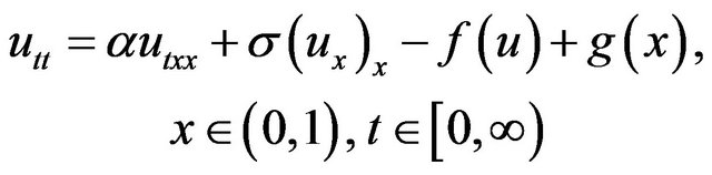
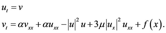
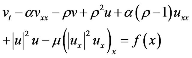
In this paper we study the initial-boundary value problem for the following nonlinear wave equation

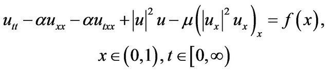(1.1)

with boundary conditions

(1.2)

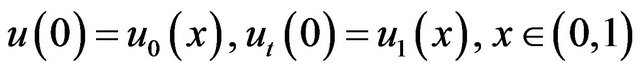
and initial conditions

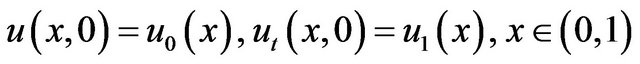(1.3)

where 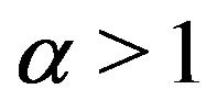constant, is a strong structural damping term, is nonlinear source term and is a nonlinear strain term.

An other version of problems (1.1)-(1.3) was studied in [1-4]. In [1] Chen et al worked that the following initial boundary value problem

(1.4)

(1.5)

(1.6)

has a global solution and there exists a compact global attractor with finite dimension. In [2] Karachalios and Staurakalis studied the local existence for (1.1) with u_t is a damping term and without nonlinear source term. In [3] Çelebi and Uğurlu gave the existence of a wide collection of finite sets of functionals on the phase space that completely determines asymptotic behavior of solutions to the strongly damped nonlinear wave equations. In [4] Chueshov presented the approach of a set of determining functionals containing determining modes and nodes that completely determines the long-time behavior of some first and second order evolution equations.

Similar results of determining modes for similar equations have been obtained in [5-7].

In this article, we take the problem defined by (1.1)- (1.3) which was not investigated in above mentioned articles. Our problem has nonlinear strain and source terms. The control of long time behavior is achieved due to the presence of restoring forces In Section 2 under conditions

and we prove the global existence and uniqueness of a weak solution u of the problems (1.1)-(1.3). In Section 3 we study determining modes on the phase space by using energy methods and the concept of the completeness defect.

2. The Global Existence and Uniqueness of Weak Solutions

Let be the usual Hilbert space of square integrable functions with the standard norm and inner product Denote 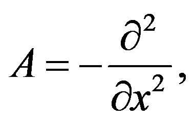the Laplacian operator on L² with domain 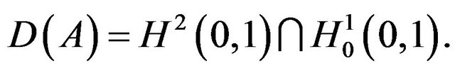A is a sectorial operator and that is a bounded linear operator defined in see [8]. The nonlinear source term satisfies the following conditions

there exists a constant such that

where Finally we denote

with the standard product norm

Define in Y by

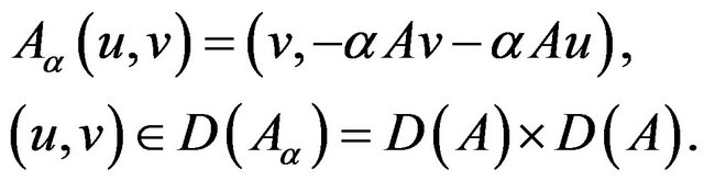(2.1)

Then the following Lemma1 is valid [9].

Lemma 1 is a sectorial operator on Y.

We define a map from to Y by

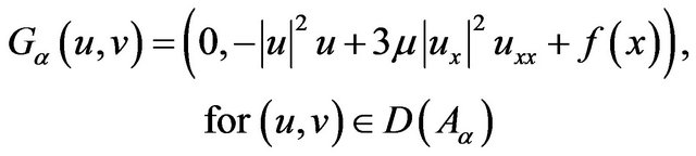(2.2)

where

Using the Sobolev embedding theorem, we can see that is locally Lipschitz continuous. Thus we apply the existence theorem in [8] to get the solutions of initial value problem for the following system in Y:

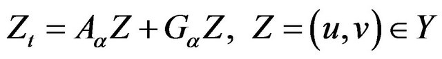(2.3)

when

(2.4)

Now, we have the following theorem.

Theorem 2 (Local existence) For and there exists such that and for a.e. and u satisfies (1.1)-(1.3). Moreover, if is maximal, then either or is unbounded on

Now for the proof of the Theorem 4 (Global Existence) we give the following Lemma 3. In the proofs of Lemma 3 and Theorem 4 (Global Existence) we repeat a similar technique used in [1].

Lemma 3 For and there exist constants

such that for

(2.5)

where u is the solution of (1.1)-(1.3).

Proof. Let where is a constant to be determined. Thus (1.1) becomes

(2.6)

Taking the inner product of both sides of (2.6) with v and integrating the resulting equation, we have

(2.7)

where

(2.8)

and

(2.9)

Now we will estimate and Choose such that

(2.10)

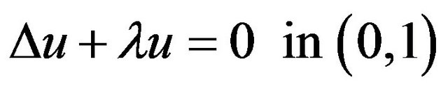
where is first eigenvalue of the following problem

From (2.8) and (2.9) with, we get

(2.11)

We use Young inequality, Poincaré inequality and (2.10) in (2.11) we find

(2.12)

Similarly, we obtain

(2.13)

Then (2.7), (2.12) and (2.13) yield

(2.14)

Using Gronwall’s inequality, we have

(2.15)

Since we can find that

by using the Sobolev embedding theorem. Thus using (2.13) in (2.15) we obtain

(2.16)

Taking

and choosing we get (2.5).■

Now we can prove the global existence of the problems (1.1)-(1.3).

Theorem 4 (Global Existence) For there exists a global solution u of problems (1.1)-(1.3) satisfying.

Proof. In Theorem 2 (Local Existence) we know that for and, for a.e. In Lemma 3 we find that and are uniformly bounded for all Now we prove the global existence of the solution u. To do this we need to show that is uniformly bounded for

Now, taking the inner product of both sides (1.1) in with, we have

(2.17)

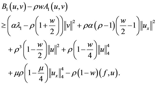
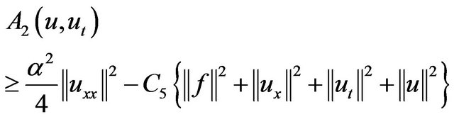
Then we multiply both sides of (2.17) by and add to (2.7) to obtain

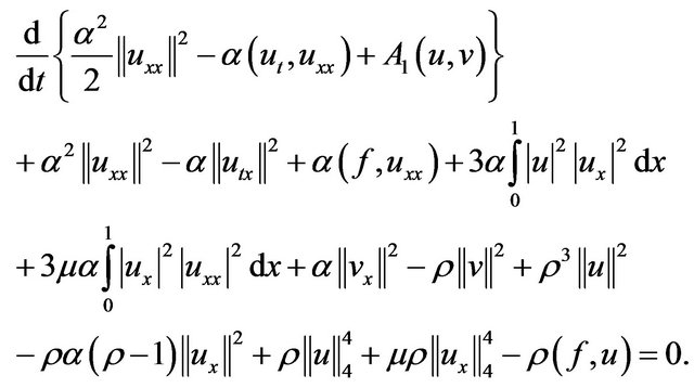(2.18)

Using Poincaré inequality and (2.10) in (2.18), we have

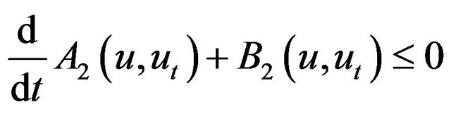(2.19)

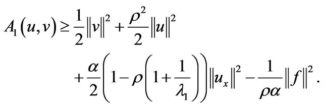
where

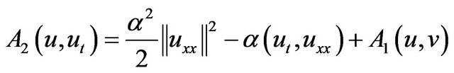(2.20)

and

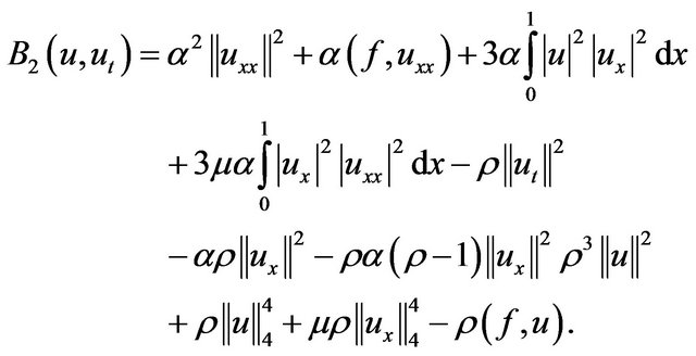(2.21)

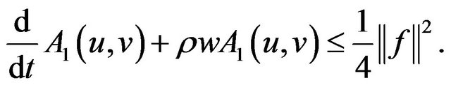
Then thanks to Young inequality we obtain

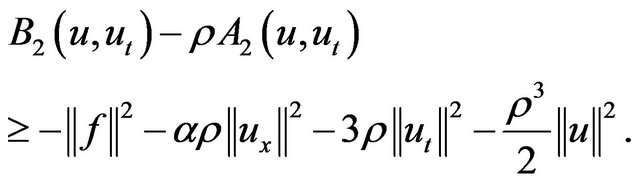(2.22)

Taking 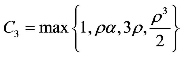in (2.22) we get

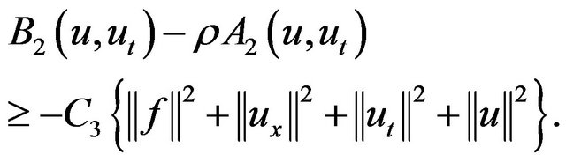(2.23)

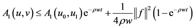
Using (2.19), (2.23) and Gronwall’s inequality we get

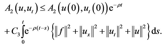(2.24)

Thus (2.24) and Lemma 3 imply that is uniformly bounded in because of

for some constant

and we have

(2.25)

where Finally, using Sobolev embedding theorem and Lemma 3 we obtain that is uniformly bounded in■

Theorem 5 (Uniqueness of weak solution) A weak solution of (1.1)-(1.3) is unique.

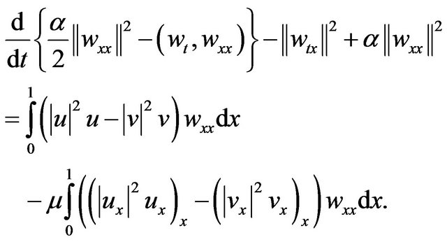
Proof. Let u and v be two distinct solutions to (1.1)- (1.3) for the same initial and boundary data. We define the difference of these solutions as Then from (1.1)-(1.3), w satisfies

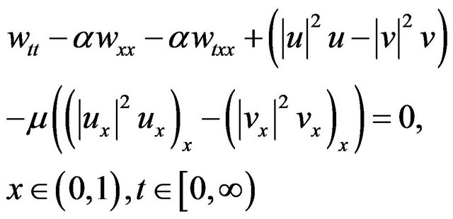(2.26)

(2.27)

(2.28)

Taking the inner product of (2.26) by in and integrating by parts gives

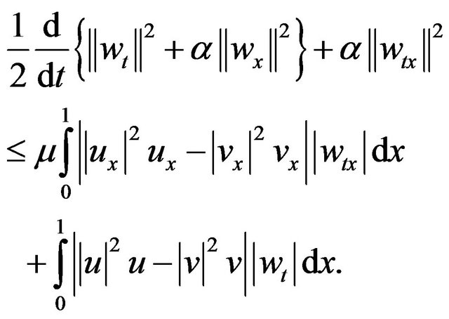(2.29)

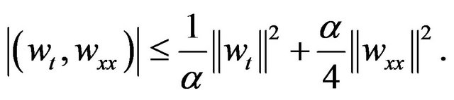
By means of the inequality

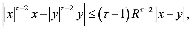(2.30)

which holds for all and it follows from (2.29) that

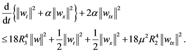
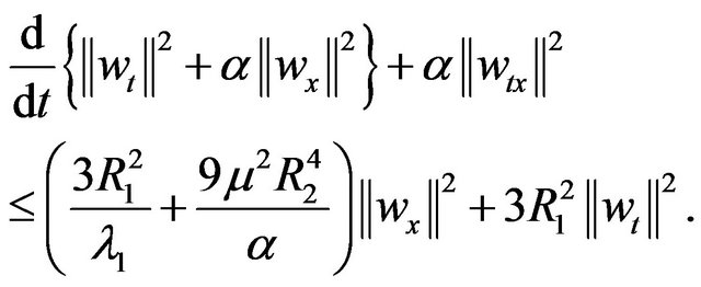(2.31)

Thus we get

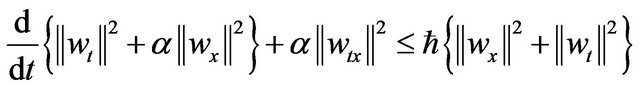(2.32)

where 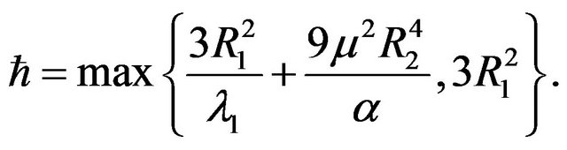Consequently the differential form of Gronwall’s inequality implies to give on■

3. Existence of Determining Functionals

Now we give some definitions, theorems and corollary for proving existence of determining functionals.

Definition 6 [4] Let be a finite set of linear continuous functionals on

We will say that is a set of determining functionals for (1.1)-(1.3) when for any two solutions with

and the conditions

(3.1)

imply

(3.2)

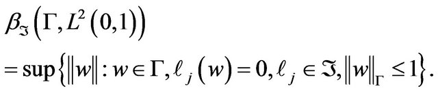
Definition 7 [4] Let V and H be the reflexive Banach spaces and V be continuously and densely embedded into H. Let be a set of linear functionals on V. We define the completeness defect of the set with respect to the pair of the spaces V and H by the formula

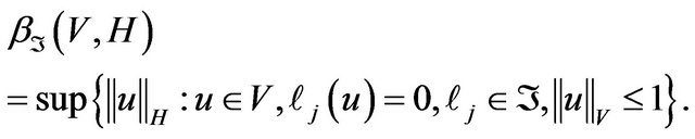(3.3)

The following assertion gives the spectral characterization of the completeness defect in the case when V and H are the Hilbert spaces.

Theorem 8 [4] Let V and H be the separable Hilbert spaces such that V is compactly and densely embedded into H. Let K be the self-adjoint, positive and compact operator in the space V defined by the equality

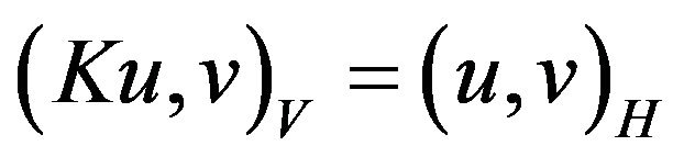
for Then the completeness defect of a set of linear functionals on V can be evaluated by the formula

where is the orthoprojector in the space V on the annihilator

is the maximal eigenvalue of the operator S.

Corollary 9 [4] Let the conditions of Theorem 8 be hold and let us denote by the orthonormal basis in the space V that consists of the eigenvectors of the operator K:

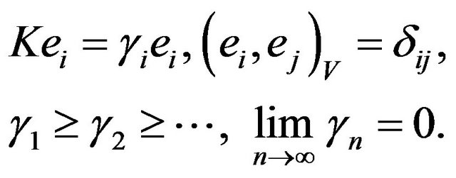(3.4)

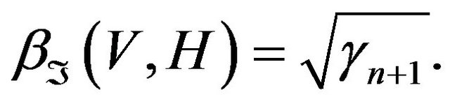
Then the completeness defect of the set of functionals,

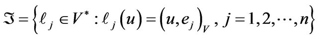
can be evaluated by the formula

The following theorem establishes a relation between the completeness defect and the set

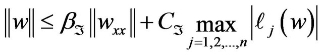
Theorem 10 [4] Let be the completeness defect of a set of linear functionals on V with respect to H. Then there exists a positive constant such that

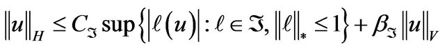(3.5)

for any where is the closed linear span of the set in the dual space of V and is the norm in

The following version of Gronwall’s lemma is also needed to determine behavior of solutions as

Lemma 11 [4] Let be a locally integrable real valued function on satisfying for some

the following conditions

(3.6)

(3.7)

where. Further, let κ be a real valued locally integrable function defined on such that

(3.8)

where Suppose that is an absolutely continuous non-negative function on such that

(3.9)

Then as

Now we can prove the main result concerning existence of a set of determining functionals of solutions to problems (1.1)-(1.3).

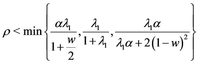
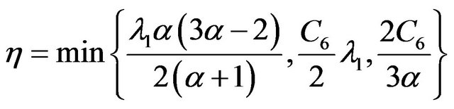
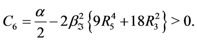
Theorem 12 Let be a set of linear continuous functionals on the space and let be a positive number satisfying

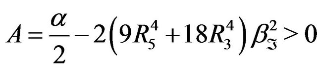where R₃, R₅ positive constants. Then, is a set of determining functionals for (1.1)-(1.3).

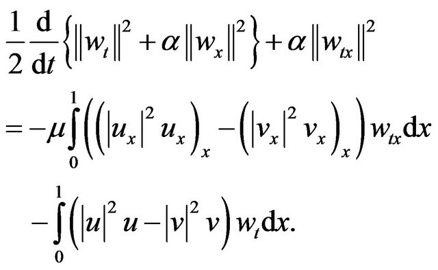
Proof. Let u and v be two solutions of problems (1.1)- (1.3). Let be the difference of these solutions. Thus w satisfies (2.26)-(2.28). Now taking the inner product of (2.26) by we get

(3.10)

Using (2.30) and Young inequality in right hand side of (3.10) we obtain

(3.11)

On the other hand, the inner product of (2.26) by and integration by parts over yields

(3.12)

We assume that for some and any small v, v₁, the nonlinear function satisfies

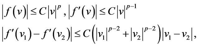(3.13)

where C is independent of v, v₁, v₂ [10]. Using (2.30) and (3.13) in (3.12) we have

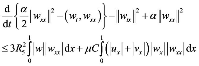(3.14)

Using the Hölder, Young and Sobolev inequalities in right hand side of (3.14) we obtain the estimate

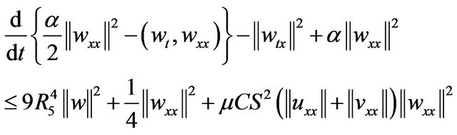(3.15)

where is the constant in the Sobolev inequality. Since there exists a positive constant D such that 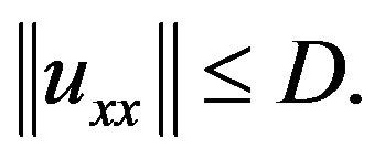Then we get

(3.16)

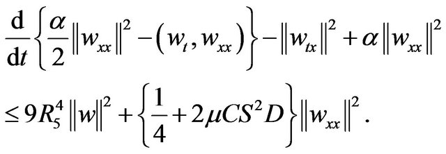
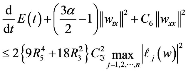
Adding (3.16) to (3.11) and using Poincaré inequality we obtain

(3.17)

where are positive constants and

.

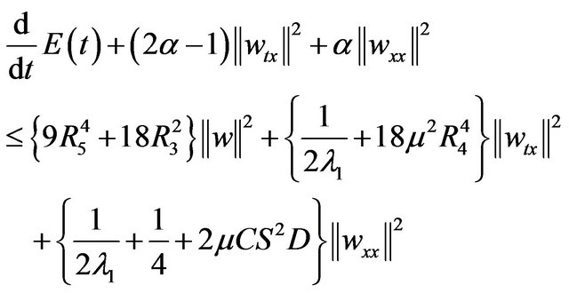
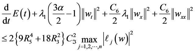
Choosing

in (3.17) leads to

(3.18)

Let denote the completeness defect between and and that is

(3.19)

From Theorem 10 we have

(3.20)

for all Squaring both sides of (3.20) and using Cauchy’s inequality we obtain

(3.21)

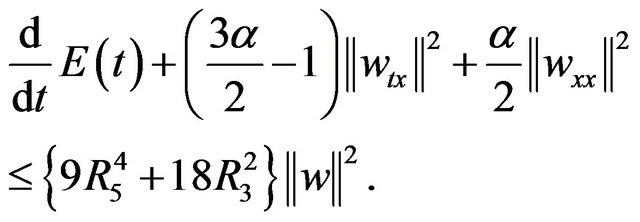
Combining (3.21) in (3.18) leads to

(3.22)

Then we choose as small as possible so that

Hence, from (3.22) we have

(3.23)

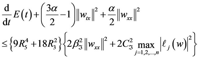
and using Poincaré inequality in (3.23) we find

(3.24)

Now we find upper and lower bounds for the functional owing to the Cauchy-Schwartz and the Cauchy inequalities:

(3.25)

Therefore, using (3.25) and from the definition of, we can find that

(3.26)

Hence, from (3.26) we can obtain that there exists a positive constant

such that

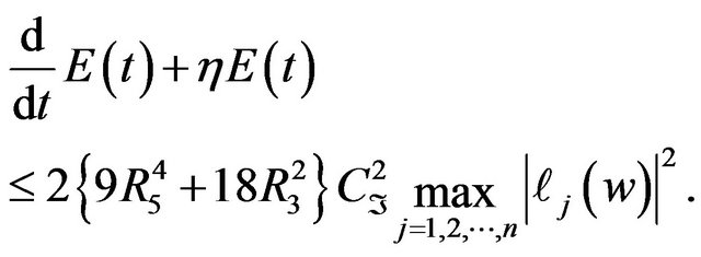(3.27)

Applying Lemma 11 to (3.27) with

and and using a result of Lemma 11 we see that if

tends to zero as then Thus we obtain that

or

As a result from Definition 6, the set defined on is a set of determining functionals for (1.1)-(1.3). Therefore we complete the proof of Theorem 12.■

4. Acknowledgements

The author thanks Professor A. Okay Çelebi for valuable hints and discussions.

REFERENCES

- F. Chen, B. Guo and P. Wang, “Long Time Behavior of Strongly Damped Nonlinear Wave Equations,” Journal of Differential Equations, Vol. 147, No. 2, 1998, pp. 231- 241. doi:10.1006/jdeq.1998.3447
- N. I. Karachalios and N. M. Staurakakis, “Global Existence and Blow up Results for Some Nonlinear Wave Equations on
,” Advances in Differential Equations, Vol. 6, No. 2, 2001, pp. 155-174.
- A. O. Çelebi and D. Uğurlu, “Determining Functionals for the Strongly Damped Nonlinear Wave Equation,” Journal of Dynamical Systems and Geometric Theories, Vol. 5, No. 2, 2007, pp. 105-116. doi:10.1080/1726037X.2007.10698530
- I. D. Chueshov, “Theory of Functionals That Uniquely Determine Long-Time Dynamics of Infinitive Dimensional Dissipative Systems,” Russian Mathematical Surveys, Vol. 53, No. 4, 1998, pp. 1-58. doi:10.1070/RM1998v053n04ABEH000057
- I. D. Chueshov and V. K. Kalantarov, “Determining Functionals for Nonlinear Damped Wave Equations,” Matematicheskaya Fizika, Analiz, Geometriya, Kharkovskii Matematicheskii Zhurnal, Vol. 8, No. 2, 2001, pp. 215- 227.
- B. Cockburn, D. A. Jones and E. S. Titi, “Determining Degrees of Freedom for Nonlinear Dissipative Systems,” Comptes Rendus de I’Académie des Sciences Paris Série I Mathématique, Vol. 321, 1995, pp. 563-568.
- J. Duan, E. S. Titi and P. Holmes, “Regularity, Approximation and Asymptotic Dynamics for a Generalized Ginzburg-Landou Equation,” Nonlinearty, Vol. 6, No. 6, 1993, pp. 915-933. doi:10.1088/0951-7715/6/6/005
- D. Henry, “Geometric Theory of Semilinear Parabolic Equations, Lecture Notes in Mathematics,” Springer-Verlag, New York, 1981.
- P. Massatt, “Limiting Behavior for Strongly Damped Nonlinear Wave Equations,” Journal of Differential Equations, Vol. 48, No. 3, 1983, pp. 334-349. doi:10.1016/0022-0396(83)90098-0
- H. Takeda and S. Yoshikawa, “On the Initial Value Problem of the Semilinear Beam Equation with Weak Damping II: Asymptotic Profiles,” Journal of Differential Equations, Vol. 253, No. 11, 2012, pp. 3061-3080.