ABSTRACT

In this paper, we present a new method, a mixture of homotopy perturbation method and a new integral transform to solve some nonlinear partial differential equations. The proposed method introduces also He’s polynomials [1]. The analytical results of examples are calculated in terms of convergent series with easily computed components [2].

1. Introduction

A new integral transform is derived from the classical Fourier integral. A new integral transform [3] was introduced by Artion Kashuri and Associate Professor Akli Fundo to facilitate the process of solving ordinary and partial differential equations in the time domain. Some integral transform method such as Laplace, Fourier, Sumudu and Elzaki transforms methods, are used to solve general nonlinear non-homogenous partial differential equation with initial conditions and use fullness of these integral transform lies in their ability to transform differential equations into algebraic equations which allows simple and systematic solution procedures. Non-linear phenomena, that appear in many areas of scientific fields such as solid state physics, plasma physics, fluid mechanics, population models and chemical kinetics, can be modeled by nonlinear differential equations. The importance of obtaining the exact or approximate solutions of nonlinear partial differential equations in physics and mathematics is still a significant problem that needs new methods to discover exact or approximate solutions. Also a new integral transform and some of its fundamental properties are used to solve general nonlinear non-homogenous partial differential equation with initial conditions. A new integral transform is defined for functions of exponential order. We consider functions in the set F defined by:

(1)

For a given function in the set, the constant must be finite number may be finite or infinite.

A new integral transform denoted by the operator is defined by the integral equation:

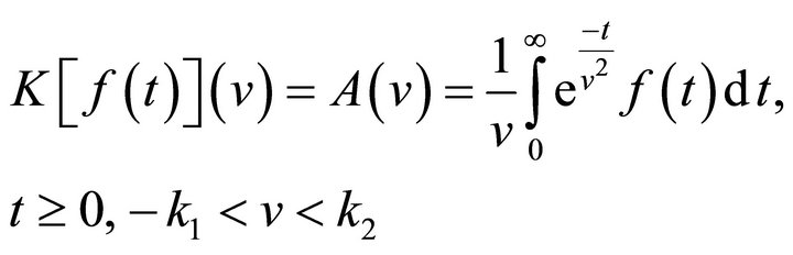(2)

A new integral transform was applied to partial differential equations, ordinary differential equations, system of ordinary and partial differential equations and integral equations. A new integral transform is a powerful tool for solving some differential equations. In this paper, we combined a new integral transform and homotopy perturbation method to solve nonlinear partial differential equations. The purpose of this study is to show the applicability and the efficiency of this mixture method. For any function, we assume that a integral Equation (2) exist.

Definition 1.1. [4] Given a function, if there is a function that is continuous on and satisfies, then we say that is the inverse new integral transform of and employ the notation,

Theorem 1.2. [Linearity of the inverse new integral

transform] Assume that exist and are continuous on and are constant coefficients. Then,

(3)

Proof. It is easy to verify that the right-hand side of first equation is a continuous function on whose a new integral transform is

Suppose that, and

. Then, and

and we know that is linear integral transform. So,

(4)

Hence,

(5)

So we have proof the theorem.                  

Theorem 1.3. [Fundamental properties of a new integral transform of partial derivatives] Let be a new integral transform of Then,

(a)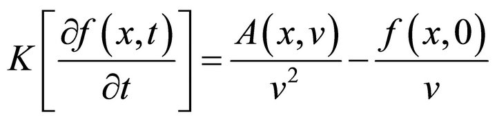

(b)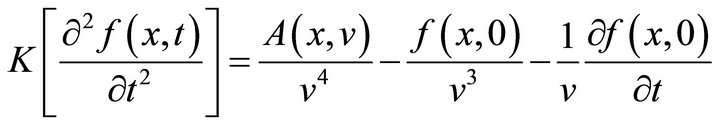

(c)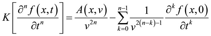

(d)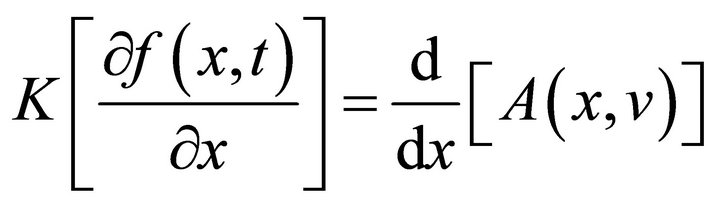

(e)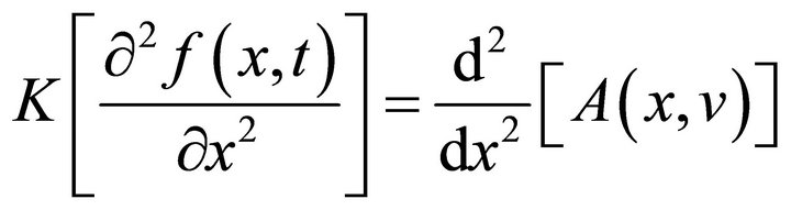

(f)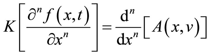

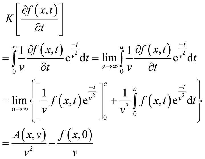
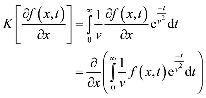
Proof. We assume that is piecewise continuous and it is of exponential order. To obtain a new integral transform of partial derivatives we use integration by parts as follows:

(a)

(b) Let substitute, 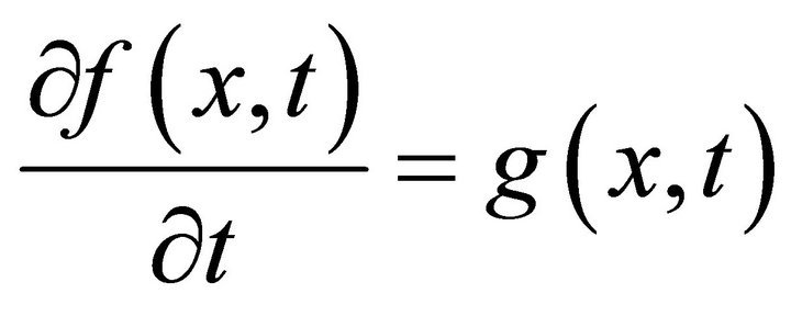then by part (a)

we have:

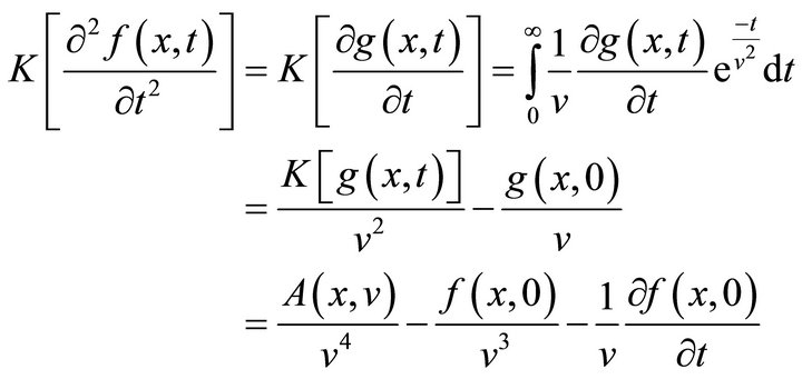
We can easily extend this result to the partial derivative by using mathematical induction to get (c).

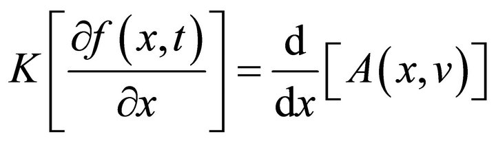
(d)

Above we have used the Leibniz’s rule to find that:

(e)

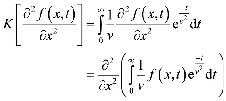
Above we have used the Leibniz’s rule to find that:

.

We can easily extend this result to the partial derivative by using mathematical induction to get (f)

So we have proof the theorem.                 

2. Homotopy Perturbation Method (HPM)

The homotopy perturbation method is considered as special case of homotopy analysis method. Let X and Y be the topological spaces. If and are continuous maps of the space X into Y, it is said that is homotopic to, if there is continuous map

such that, and

for each. The map G is called homotopy between and. To explain the homotopy perturbation method, we consider a general equation of the type,

(6)

where is any differential operator. We define a convex homotopy by,

(7)

where is a functional operator with known solution which can be obtained easily. It is clear that, for

we have,

. In topology this show that continuously traces an implicitly defined curve from a starting point to a solution function

.

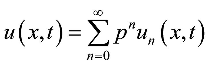
The uses the embedding parameter as an expanding parameter [1,5] and write the solution as a power series:

(8)

If then (8) corresponds to (7) and becomes the approximate solution of the form,

(9)

The embedding parameter monotonically increases from zero to unit, so as the trivial problem

is continuously deforms the original problem

. It is well known that the series (8) is convergent for most of the cases and also the rate of convergence is depending on. We assume that (9) has a unique solution. The comparisons of like powers of give solutions of various orders.

Mixture of a New Integral Transform and (HPM)

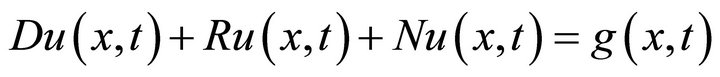
Consider a general nonlinear non-homogenous partial differential equation with initial conditions of the form:

(10)

where D is linear differential operator of order two, is linear differential operator of less order than, is the general nonlinear differential operator and is the source term. Taking a new integral transform on both sides of equation (10) we get:

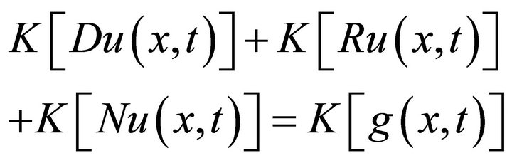(11)

Using the differentiation property of a new integral transform by theorem (1.3) and above initial conditions, we have:

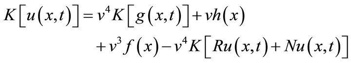(12)

Applying the inverse new integral transform on both sides of Equation (12) we find:

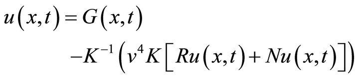(13)

where represents the term arising from the source term and the prescribed initial conditions. Now, we apply the homotopy perturbation method.

(14)

and the nonlinear term can be decomposed as,

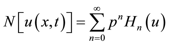(15)

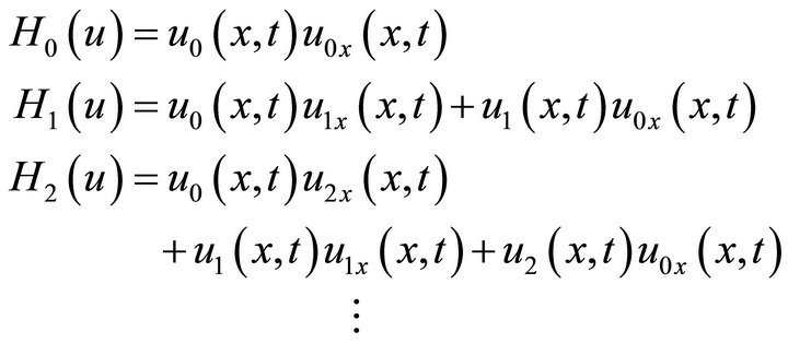
where are the so-called He’s polynomials [1] that represents the nonlinear terms and are given by the formula:

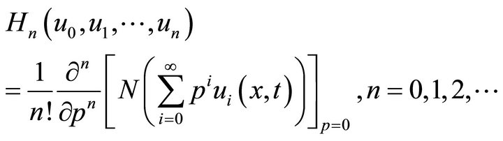(16)

Substituting Equations (14) and (15) in Equation (13) we get:

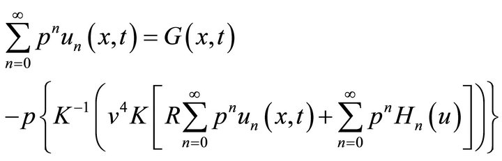(17)

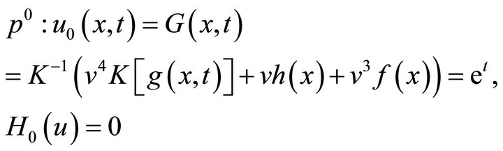
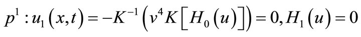
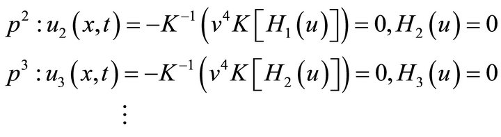
This is the coupling of a new integral transform and the homotopy perturbation method [5]. Comparing the coefficients of like powers of p, the following approximations are obtained:

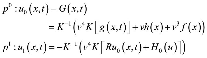
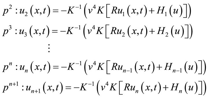
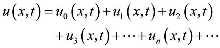
Then the solution is :

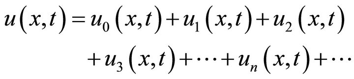(18)

It is worth mentioning that the method is capable of reducing the volume of the computational work as compared to the classical methods while still maintaining the high accuracy of the numerical result and no requirement to complicated calculations. The size reduction amounts to an improvement of the performance of the approach.

3. Applications

Application of the mixture of a new integral transform and homotopy perturbation method for solving nonlinear partial differential equations. In this section we apply the homotopy perturbation method and a new integral transform method in order to get the solution procedure of this.

The following examples illustrate the use of this new mixture method in solving certain initial value problems described by nonlinear partial differential equations.

Example 3.1.

Consider the following non-homogenous nonlinear partial differential equation with initial conditions:

(19)

(20)

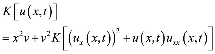
By applying a new integral transform of Equation (19) subject to the initial conditions (20) we have:

(21)

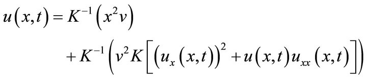
The inverse new integral transform implies that,

(22)

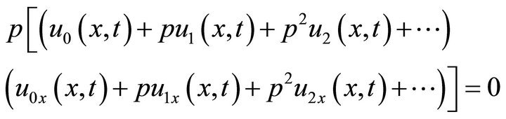
Now applying the homotopy perturbation method in Equation (22) we get:

(23)

where are He’s polynomials that represents the nonlinear terms. Then,

(24)

where,

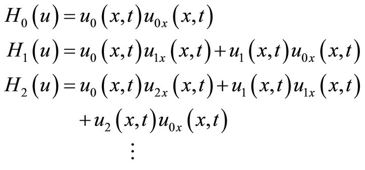
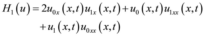
The first few components of are given by:

(25)

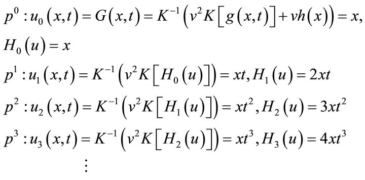
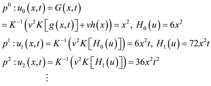
Comparing the coefficients of the same powers of, we get:

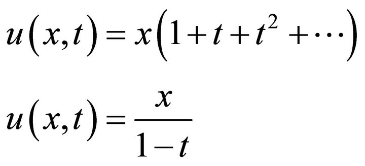
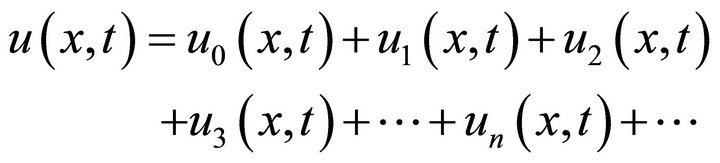
Then the solution is:

(26)

Example 3.2.

Consider the following non-homogenous nonlinear partial differential equation with initial conditions:

(27)

(28)

By applying a new integral transform of Equation (27) subject to the initial conditions (28) we have:

(29)

The inverse new integral transform implies that,

(30)

Now applying the homotopy perturbation method in Equation (30) we get:

(31)

where are He’s polynomials that represents the nonlinear terms. Then,

(32)

where,

The first few components of are given by:

(33)

Comparing the coefficients of the same powers of, we get:

Then the solution is:

(34)

Example 3.3.

Consider the following homogenous nonlinear partial differential equation with initial condition:

(35)

(36)

By applying a new integral transform of Equation (35) subject to the initial condition (36) we have:

(37)

The inverse new integral transform implies that,

(38)

Now applying the homotopy perturbation method in Equation (38) we get:

(39)

where are He’s polynomials that represents the nonlinear terms. Then,

(40)

where,

The first few components of are given by:

(41)

Comparing the coefficients of the same powers of, we get:

Then the solution is:

(42)

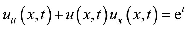
Example 3.4.

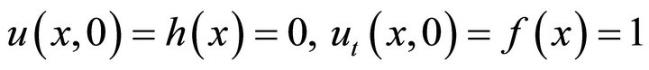
Consider the following homogenous nonlinear partial differential equation with initial condition:

(43)

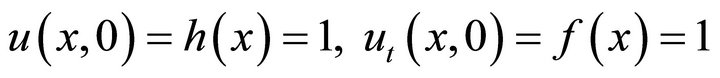
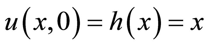
(44)

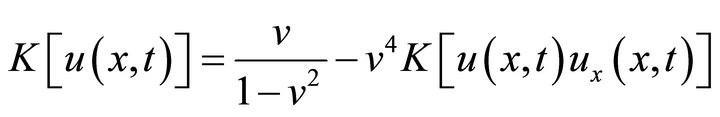
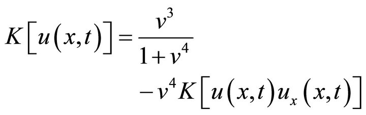
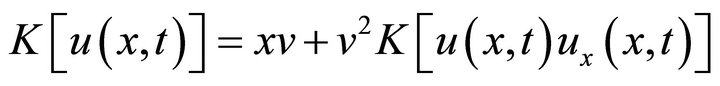
By applying a new integral transform of Equation (43) subject to the initial condition (44) we have:

(45)

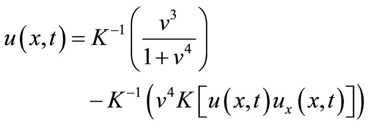
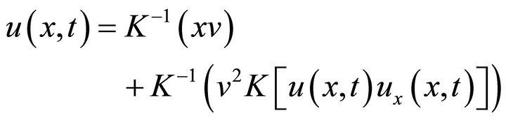
The inverse new integral transform implies that,

(46)

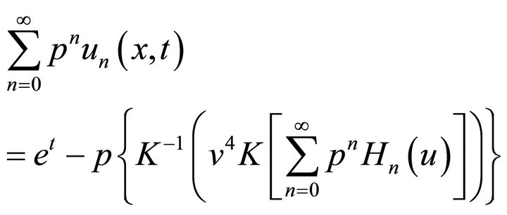
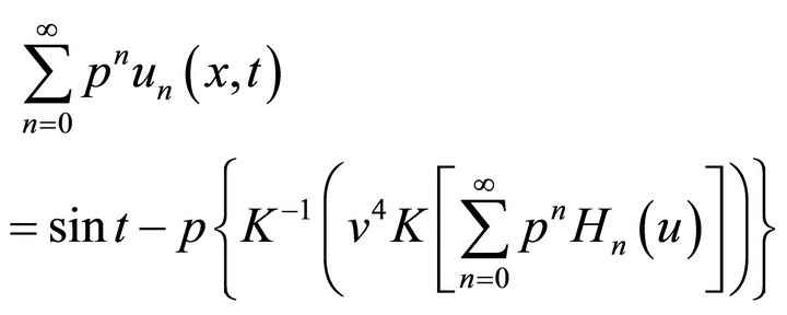
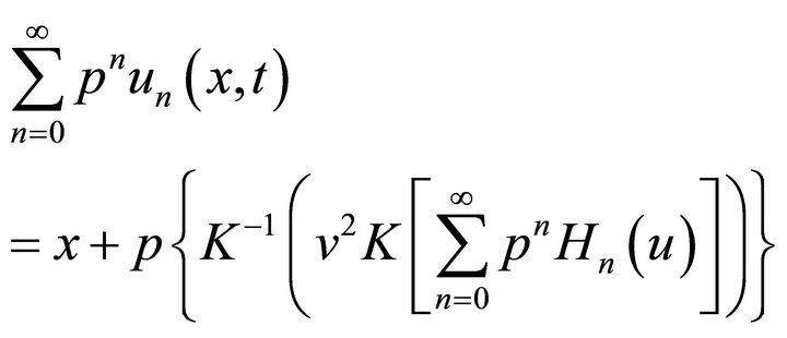
Now applying the homotopy perturbation method in Equation (46) we get:

(47)

where are He’s polynomials that represents the nonlinear terms. Then,

(48)

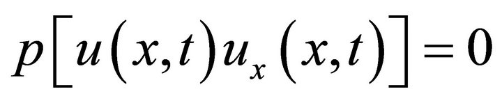
where,

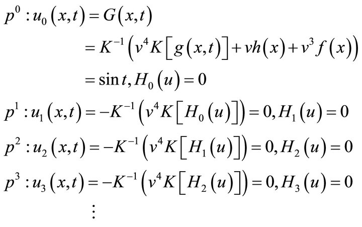
The first few components of are given by:

(49)

Comparing the coefficients of the same powers of, we get:

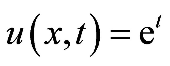
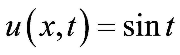
Then the solution is:

(50)

4. Conclusion

In this paper, we mixture a new integral transform and homotopy perturbation method to solve nonlinear partial differential equations. The solution of four nonlinear partial differential equations with initial conditions is presented by using this method and simple calculation of He’s polynomials. It is worth mentioning that the method is capable of reducing the volume of the computational work as compared to the classical methods while still maintaining the high accuracy of the numerical result and no requirement to complicated calculations. The size reduction amounts to an improvement of the performance of the approach.

REFERENCES

- E. M. E. Zayed and H. M. Abdel Rahman, “On Using the He’s Polynomials for Solving the Nonlinear Coupled Evolution Equations in Mathematical Physics,” WSEAS Transactions on Mathematics, Vol. 11, No. 4, 2012, pp. 294-302.
- D. Kumar, J. Singh and S. Rathore, “Sumudu Decomposition Method for Nonlinear Equations,” International Mathematical Forum, Vol. 7, No. 11, 2012, pp. 515-521.
- A. Kashuri and A. Fundo, “A New Integral Transform,” Advances in Theoretical and Applied Mathematics, Vol. 8, No. 1, 2013, pp. 27-43.
- R. K. Nagle, E. B. Saff and A. D. Snider, “Fundamentals of Differential Equations,” 8th Edition, Pearson, London, 2011, p. 367.
- T. M. Elzaki and E. M. A. Hilal, “Homotopy Perturbation and Elzaki Transform for Solving Nonlinear Partial Differential Equations,” Mathematical Theory and Modeling, Vol. 2, No. 3, 2012, pp. 33-43.