World Journal of Mechanics
Vol.05 No.11(2015), Article ID:61135,12 pages
10.4236/wjm.2015.511021
Elastic Stress Predictor for Stochastic Finite Element Problems
Drakos Stefanos
International Center for Computational Engineering, Rhodes, Greece

Copyright © 2015 by author and Scientific Research Publishing Inc.
This work is licensed under the Creative Commons Attribution International License (CC BY).
http://creativecommons.org/licenses/by/4.0/


Received 8 October 2015; accepted 13 November 2015; published 16 November 2015
ABSTRACT
The paper presents a new algorithm of elastic stress predictor in non linear stochastic finite element method using the Generalized Polynomial Chaos. The statistical moments of strains calculated based on the displacement Polynomial Chaos expansion. To descretise the stochastic process of material the Karhunen-Loeve Expansion was used and it is presented. Using the strains and the material Karhunen-Loeve Expansion the stress components are calculated. A numerical example of shallow foundation was carried out and the results of stress and strain of the new algorithm were compared with those raised from Monte Carlo method which is treated as the exact solution. A great accuracy was presented.
Keywords:
Polynomial Chaos, Stochastic Finite Element, Karhunen-Loeve Expansion, Quantification of Uncertainty

1. Introduction
The analysis and design in structural and geotechnical engineering problems requires the calculation of stress and strain which is generally a difficult task because of the uncertainty and spatial variability of the materials’ properties. Various forms of uncertainties arise which depend on the nature of geological formation or construction method, the site investigation, the type and the accuracy of design calculations etc. In recent years there has been considerable interest amongst engineers and researchers in the issues related to quantification of uncertainty as it affects safety, design as well as the cost of projects [1] - [4] .
A number of approaches using statistical concepts have been proposed in engineering in the past 25 years or so. These include the Stochastic Finite Element Method (SFEM) [5] - [7] , and the Random Finite Element Method (RFEM) [8] - [12] . The RFEM involves generating a random field of soil or structure properties with controlled mean, standard deviation and spatial correlation length, which is then mapped onto a finite element mesh. However the number of works on the stochastic stress and strain calculation and their statistical moments are limited. An essential paper on the field is presented by Ghosh & Farhat [13] where the constitutive relation of stress and strain calculated by different approaches.
In this paper we present SFEM [14] - [18] using the method of Generalized Polynomial Chaos (GPC) [19] . To descretise the stochastic process of material the Karhunen-Loeve Expansion was used and it is presented. The constitutive relation of stress and strain calculated using the Generalized Polynomial Chaos and verified against Monte Carlo simulation which is treated as the exact solution based on a series of computational experiment. In order to solve an elastoplastic problem the invariants of stress are also needed. In the current work the stochastic stress invariants are given also.
A numerical example of shallow foundation is given in the last part of the paper. The results of the two methods of stress and strains calculation are compared and presented.
2. Probability Density Definition
Considering an arbitrary body and a the sample space  where
where  is the σ-algebra and is considered to contain all the information that is available,
  is the probability measure and the spatial domain of the body is
 . Assuming that the parameters of the body
  for
for  and
and  dependent on a finite
number M of random variables  and
and . To compute the
statistical moments of the results we perform a change of variable  and
and  [20] . If ρ is the joint density and random variables are independent and
  denote the density of
  then:
then:
 (1)
(1)
The expected value of a quantity of the problem is given by the following norm:
 (2)
(2)
3. Computation of Strains
The author has presented a stochastic finite element procedure to solve boundary problems using polynomial chaos [15] - [18] . The outcome displacement of the problem is given by the polynomial chaos expansion as:
 (3)
(3)
where the order Q and the formula  of Polynomial Chaos are given in Appendix A.
In order to propagate the uncertainties from input parameters to the results for an elastoplastic problem throw the constitutive equation the strains must be calculated first.
In an elastostatic problem of homogeneous isotropic body one of the field equations that must be satisfied at all interior points of the body is the Strain-Displacement relations:
 (4)
(4)
Using the displacement polynomial chaos expansion the Equation (4) leads to:
 (5)
(5)
4. Integration Algorithm
Solving for each increment the boundary problem the strain Polynomial Chaos Expansion can be calculated as before. At each increment n + 1 they are also known the stress from the previous state  the plastic strain
 . The basic steps in computing the new state of stress are as follows:
The mean value of elastic predictor and of the trial stress are given:
 (6)
(6)
 (7)
(7)
The 4th-order stochastic elasticity tensor of elastic module is given by the equation:
 (8)
(8)
 : is expressed in terms of (deterministic) Poisson’s ratio as
 (9)
(9)
Based on that the stochastic process of Young modulus over the spatial domain with a known mean value  and covariance matrix
  assuming lognormal distribution the Karhunen-Loeve expansion has been used which is the most efficient method for the discretization of a random field. Thus:
 (10)
(10)
where:
 : is the eigenvalues of the covariance function;
 : is the eigenfunctions of the covariance function
5. Constitutive Equations for Plain Strain Condition
Assuming one dimension and 3rd order polynomial chaos and plain strain conditions:
 (11)
(11)
Considering as ,
,  and
and  the mean value the standard deviation and the coefficient of variation
of Elasticity modulus , the mean values and the variance of the lognormal distribution are equal to:
 (12)
(12)
Using the Chaos polynomial expansion the stochastic equation of each component of stress is given:
 (13)
(13)
The expected value after some algebra gives:
 (14)
(14)
The variance of stress:
 (15)
(15)
where:
 (16)
(16)
Similarly for the other components.
Expected value of :
:
 (17)
(17)
Based on the stochastic Equation (13) of  components the expected value of the invariant
  is given as following:
 (18)
(18)
 (19)
(19)
 (20)
(20)
Variance value of :
:
Using again the stochastic Equation (13) of  components the variance of
 :
:
 (21)
(21)
where:
 (22)
(22)
As an example the variance of  is given:
 (23)
(23)
The expected value of :
:
 (24)
(24)
The variance value of :
:
 (25)
(25)
The analysis are carried out similar as the invariant of .
.
6. Numerical Example
A shallow foundation problem for various values of variation’s coefficient  is solved taken to account the randomness of the ground. To estimate the statistical moments of the soil deformation the numerical algorithm of SFEM using the Generalized Polynomial Chaos as described in the previous paragraphs is applied. In [16] the author compared the displacement results to those obtained by the closed form solution.
The geometry of the finite elements used for the simulation of the problem presented in Figure 1. The input data of the problem is the random field modulus with a constant average value equal to 100 Mpa and a fixed
Poisson ratio equal to 0.25. Calculations have been made for ten different coefficients  of the elastic
modulus with a minimum value of 0.1 and then with step 0.1 to a maximum value equal to 1. For SFEM one dimensional Hermite GPC with order 5 [19] were used. In the Figures B1-B10 (Appendix B), the strains and stress components, and the stress tensor invariants are presented as resulted by the Chaos Polynomial expansion (Appendix A) and compared with those raised by the Monte Carlo Method. The convergence of the outcomes decreases as the number of Monte Carlo simulations increases.
7. Conclusions
To propagate the uncertainties of input parameters to constitutive relations of strain and stress where arises due
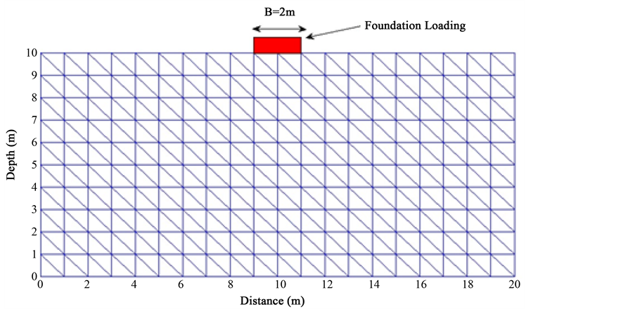
Figure 1. Finite element mesh.
to spatial variability of mechanical parameters in engineering problems, a new algorithm of Stochastic Finite Element Method has been presented.
An algorithm of Stochastic Finite Element using Polynomial Chaos has been developed and the elastic predictor of stress in a non linear problem is calculated.
A numerical example of shallow foundation was carried out and the results of stress and strain of the new algorithm were compared with those raised from Monte Carlo method which is treated as the exact solution. A great accuracy was presented.
The main advantage in using the proposed methodology is that a large number of realizations which have to be made for (Random Finite Element Method) avoided, thus making the procedure viable for realistic practical problems.
Cite this paper
Drakos Stefanos, (2015) Elastic Stress Predictor for Stochastic Finite Element Problems. World Journal of Mechanics,05,222-233. doi: 10.4236/wjm.2015.511021
References
- 1. Hasselman, T. (2001) Quantification of Uncertainty in Structural Dynamic Models. Journal of Aerospace Engineering, 14, 158-165.
http://dx.doi.org/10.1061/(ASCE)0893-1321(2001)14:4(158) - 2. Preis, A., Perelman, L. and Ostfeld, A. (2008) Uncertainty Quantification of Contamination Source Identification. World Environmental and Water Resources Congress 2008, 1-6.
http://dx.doi.org/10.1061/40976(316)505 - 3. Keitel, H. (2013) Quantifying Sources of Uncertainty for Creep Models under Varying Stresses. Journal of Structural Engineering, 139, 949-956.
http://dx.doi.org/10.1061/(ASCE)ST.1943-541X.0000716 - 4. Karim, A., Ahmed, I., Boutton, T., Strom, K. and Fox, J. (2015) Quantification of Uncertainty in a Sediment Provenance Model. World Environmental and Water Resources Congress 2015, 1790-1799.
http://dx.doi.org/10.1061/9780784479162.175 - 5. Phoon, K., Quek, S., Chow, Y. and Lee, S. (1990) Reliability Analysis of Pile Settlements. Journal of Geotechnical Engineering, ASCE, 116, 1717-35.
http://dx.doi.org/10.1061/(ASCE)0733-9410(1990)116:11(1717) - 6. Mellah, R., Auvinet, G. and Masrouri, F. (2000) Stochastic Finite Element Method Applied to Non-Linear Analysis of Embankments. Probabilistic Engineering Mechanics, 15, 251-259.
http://dx.doi.org/10.1016/S0266-8920(99)00024-7 - 7. Eloseily, K., Ayyub, B. and Patev, R. (2002) Reliability Assessment of Pile Groups in Sands. Journal of Structural Engineering, ASCE, 128, 1346-53.
http://dx.doi.org/10.1061/(ASCE)0733-9445(2002)128:10(1346) - 8. Fenton, G.A. and Vanmarcke, E. H. (1990) Simulation of Random Fields via Local Average Subdivision. Journal of Engineering Mechanics, 116, 1733-1749.
http://dx.doi.org/10.1061/(ASCE)0733-9399(1990)116:8(1733) - 9. Paice, G.M., Griffiths, D.V. and Fenton, G.A. (1996) Finite Element Modeling of Settlements on Spatially Random Soil. Journal of Geotechnical Engineering, 122, 777-779.
http://dx.doi.org/10.1061/(ASCE)0733-9410(1996)122:9(777) - 10. Fenton, G.A. and Griffiths, D.V. (2002) Probabilistic Foundation Settlement on Spatially Random Soil. Journal of Geotechnical and Geoenvironmental Engineering, 128, 381-390.
http://dx.doi.org/10.1061/(ASCE)1090-0241(2002)128:5(381) - 11. Fenton, G.A. and Griffiths, D.V. (2005) Three-Dimensional Probabilistic Foundation Settlement. Journal of Geotechnical and Geoenvironmental Engineering, 131, 232-239.
http://dx.doi.org/10.1061/(ASCE)1090-0241(2005)131:2(232) - 12. Fenton, G.A. and Griffiths, D.V. (2008) Risk Assessment in Geotechnical Engineering. Wiley, Hoboken.
http://dx.doi.org/10.1002/9780470284704 - 13. Debraj, G. and Charbel, F. (2008) Strain and Stress Computations in Stochastic Finite Element Methods. International Journal for Numerical Method in Engineering, 74, 1219-1239.
http://dx.doi.org/10.1002/nme.2206 - 14. Ghanem, R.G. and Spanos, P.D. (1991) Stochastic Finite Elements: A Spectral Approach. Springer-Verlag, New York.
http://dx.doi.org/10.1007/978-1-4612-3094-6 - 15. Drakos, I.S. and Pande, G.N. (2015) Stochastic Finite Element Analysis for Transport Phenomena in Geomechanics Using Polynomial Chaos. Civil and Structural Engineering, GJRE-E, Vol. 15, Issue 2, Version 1.0.
- 16. Drakos, I.S. and Pande, G.N. (2015) Quantitative of Uncertainties in Earth Structures. World Congress on Advances in Structural Engineering and Mechanics, Incheon, 25-29 August 2015, 25-29.
- 17. Drakos, I.S. and Pande, G.N. (2015) Stochastic Finite Element Analysis Using Polynomial Chaos. Studia Geotechnica et Mechanica Journal. (under review)
- 18. Drakos, I.S. and Pande, G.N. (2015) Stochastic Finite Element Consolidation Analysis Based on Polynomial Chaos Expansion. Georisk Journal. (under review)
- 19. Xiu, D.B. and Em Karniadakis, G. (2003) Modeling Uncertainty in Steady State Diffusion Problems via Generalized Polynomial Chaos. Computer Methods in Applied Mechanics and Engineering, 191, 4927-4948.
http://dx.doi.org/10.1016/S0045-7825(02)00421-8 - 20. Lord, G., Powel, C. and Shardlow, T. (2014) An Introduction to Computational Stochastic PDEs. Cambridge Texts in Applied Mathematics. Cambridge University Press, Cambridge.
http://dx.doi.org/10.1017/cbo9781139017329
Apendix A
Galerkin Approximation and Generalized Polynomial of Chaos
In order to solve the problem we have to create the new space . For that reason the subspace
  is considered as [20] .
 (A.1)
(A.1)
Assuming that the  represents a space of univariate orthonormal polynomial of variable
  with order k or lower and:
 (A.2)
(A.2)
The tensor product of the M  subspace results the space of the Generalized Polynomial Chaos:
 (A.3)
(A.3)
And using (A2)
 (A.4)
(A.4)
where 
And
 (A.5)
(A.5)
Xiu & Karniadakis [19] show the application of the method for different kind of orthonormal polynomials and in the current paper the Hermite polynomial was used with the following characteristics:

 (A.6)
(A.6)
where:
 : are the normalization factors,
  is the Kronecker delta;
 : is the density function and
For a 3rd order of one dimension of uncertainty the Hermite Polynomial Chaos is given by:
 (A.7)
(A.7)
Apendix B
Results of Numerical Example

Figure B1. Expected value of stress tensor complements.
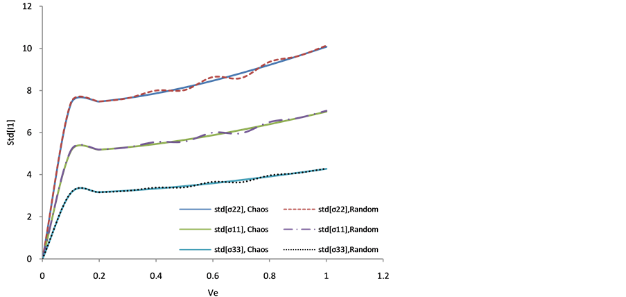
Figure B2. Standard deviation of stress tensor complements.
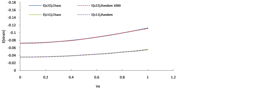
Figure B3. Expected value of strain tensor complements.
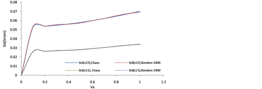
Figure B4. Standard deviation of strain tensor complements.

Figure B5. Expected value of stress tensor invariant I1.

Figure B6. Standard deviation of stress tensor invariant I1.

Figure B7. Expected value of stress tensor invariant I2.

Figure B8. Standard deviation of stress tensor invariant I2.

Figure B9. Expected value of stress tensor invariant I3.

Figure B10.Standard deviation of stress tensor invariant I3.