World Journal of Mechanics
Vol. 3 No. 2 (2013) , Article ID: 30859 , 11 pages DOI:10.4236/wjm.2013.32008
Structural Reliability Assessment by a Modified Spectral Stochastic Meshless Local Petrov-Galerkin Method
1Department of Accounting and Information System, Chang-Jung Christian University, Tainan, Chinese Taipei
2Department of Civil Engineering, Feng-Chia University, Taichung, Chinese Taipei
Email: xsheu@hotmail.com
Copyright © 2013 Guang Yih Sheu. This is an open access article distributed under the Creative Commons Attribution License, which permits unrestricted use, distribution, and reproduction in any medium, provided the original work is properly cited.
Received January 29, 2013; revised March 9, 2013; accepted March 16, 2013
Keywords: Spectral Stochastic Meshless Local Petrov-Galerkin Method; Generalized Polynomial Chaos Expansion; First-Order Reliability Method; Structural Failure Probability; Reliability Index
ABSTRACT
This study presents a new tool for solving stochastic boundary-value problems. This tool is created by modify the previous spectral stochastic meshless local Petrov-Galerkin method using the MLPG5 scheme. This modified spectral stochastic meshless local Petrov-Galerkin method is selectively applied to predict the structural failure probability with the uncertainty in the spatial variability of mechanical properties. Except for the MLPG5 scheme, deriving the proposed spectral stochastic meshless local Petrov-Galerkin formulation adopts generalized polynomial chaos expansions of random mechanical properties. Predicting the structural failure probability is based on the first-order reliability method. Further comparing the spectral stochastic finite element-based and meshless local Petrov-Galerkin-based predicted structural failure probabilities indicates that the proposed spectral stochastic meshless local Petrov-Galerkin method predicts the more accurate structural failure probability than the spectral stochastic finite element method does. In addition, generating spectral stochastic meshless local Petrov-Galerkin results are considerably time-saving than generating Monte-Carlo simulation results does. In conclusion, the spectral stochastic meshless local Petrov-Galerkin method serves as a time-saving tool for solving stochastic boundary-value problems sufficiently accurately.
1. Introduction
Available stochastic numerical methods for solving stochastic boundary-value problems include the Monte Carlo simulation, spectral stochastic finite element [1] and stochastic element-free Galerkin methods [2]. The Monte Carlo simulation may be simplest, since implementing it requires sampling the existing random fields and substituting the resulting samples into deterministic solutions. However, a perquisite of obtaining accurate Monte Carlo simulation results is sufficiently sampling the existing random fields; therefore, completing a Monte Carlo simulation is usually time-consuming. This perquisite brings about a motive of developing a time-saving tool for solving stochastic boundary-value problems.
Meanwhile, the spectral stochastic finite element or stochastic element-free Galerkin methods are developed by extending the finite element or element-free Galerkin methods. For example, deducing a spectral stochastic finite element couples a finite element formulation with such as polynomial chaos and Karhunen-Loève expansions of stochastic processes. These stochastic processes are assumed to represent the existing uncertainty.
A number of spectral stochastic finite element formulations are available for some branches in engineering science and mechanics. References [3,4] are two recent examples. Nevertheless, applying these two stochastic numerical methods needs a finite element discretization or background cells for the numerical integration. To provide more freedom in solving stochastic boundary-value problems, a truly-meshless stochastic numerical method may be a promising alternative. In a published study [5], a spectral stochastic meshless local Petrov-Galerkin method has been developed by coupling a meshless local Petrov-Galerkin formulation and radial basis functionbased meshfree shape functions with polynomial chaos expansions [6] of stochastic processes. Since the meshless local Petrov-Galerkin method is truly meshless [7], the spectral stochastic meshless local Petrov-Galerkin method is also truly meshless. Nonetheless, the spectral stochastic meshless local Petrov-Galerkin results of two elastostatic problems are more accurate than spectral stochastic finite element results of the same problems. In addition, generating the spectral stochastic meshless local Petrov-Galerkin results is considerably time-saving.
Based on the published conclusion [8] that the MLPG5 scheme may substitute for the finite element method to solve boundary-value problems, the current study further derives a two-dimensional spectral stochastic meshless local Petrov-Galerkin formulation in elastostatics using the MLPG5 scheme. The resulting spectral stochastic meshless local Petrov-Galerkin formulation is selectively applied to predict the structural failure probability with the uncertainty in the spatial variability of mechanical properties. In addition to the MLPG5 scheme, deriving the proposed spectral stochastic meshless local PetrovGalerkin formulation adopts the generalized polynomial chaos expansions [6] of random mechanical properties and radial basis function-based meshless shape functions. Meanwhile, predicting the structural failure probability is based on the first-order reliability method [9].
The remainder of this study is organized in 5 sections. In Section 2, deriving a meshless local Petrov-Galerkin formulation in elastostatics using the MLPG5 scheme is presented. In Section 3, coupling the resulting expressions in Section 2 with generalized polynomial chaos expansions of random mechanical properties to deduce a spectral stochastic meshless local Petrov-Galerkin formulation is presented. In Section 4, the algorithm for implementing the first-order reliability method is reviewed. Section 5 inspects the accuracy of spectral stochastic meshless local Petrov-Galerkin-based results. Based on this inspection, Section 6 presents the conclusion.
2. Meshless Local Petrov-Galerkin Formulation
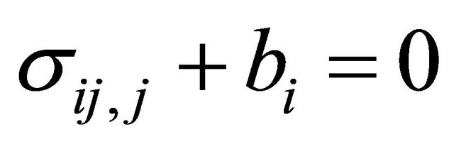
Suppose the linearly elastic and isotropic material. In addition, the infinitesimal strain assumption holds. Describe any physical parameter as functions of x and q within a problem domain W in which x = (x1, x2) is a vector of spatial coordinates and q is an event in the probability space. The succeeding study introduces the stress equations of equilibrium to derive a meshless local Petrov-Galerkin formulation. These stress equations have the following tensor form [10]:
 (1)
(1)
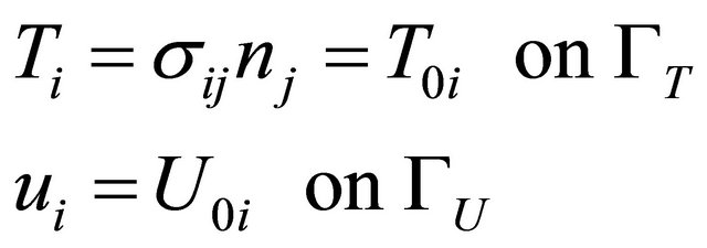
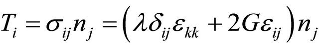
where (×),j = ¶(×)/¶xj, sij is the stress field corresponding to the displacement field ui (i = 1 to 2) and bi is the body force. The boundary conditions are
 (2)
(2)
where GT is the natural boundary, GU is the essential boundary, Ti are the tractions, U0i and T0i are known functions, nj are the components of a unit vector n outward normal to G, and G = GUUGT.
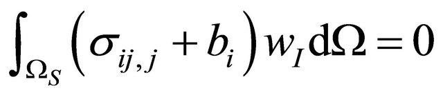
If NT nodes locate within W and WS represents a local quadrature domain for a node xI (I = 1 to NT), a local weak form of Equation (1) is
 (3)
(3)
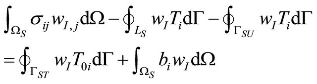
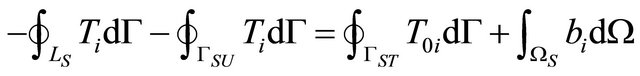
where wI is the test function associated with xI. Subsequently, this study similarly manipulates a published radial basis function-based interpolation formula [5] to construct the meshfree shape function N. Since the resulting N satisfies the Kronecker delta function property (dIJ = 0 for I ¹ J, dIJ = 1 for I = J, and I, J denote the I-th and J-th nodes), Equation (3) contains neither Lagrangian multipliers nor penalty parameters for imposing the essential boundary condition. Further simplifying Equation (3) by the divergence theorem results in
 (4)
(4)
where GST = WSIGT, GSU = WSIGU, LS = GS – GST – GSU, and GS is the boundary of WS. Theoretically speaking, the shape of WS can be arbitrary in computing Equation (4). However, choosing each WS as a rectangular centered at xI (I = 1 to NT) can simplify the numerical integration of Equation (4). In addition, WS for xI (I = 1 to NT) may be different from an interpolation domain WQ for approximating an unknown or a random field in the neighborhood of the same node. The difference between WS and WQ is further illustrated in Figure 1. Also different in terpolation domains or points may be chosen for approximating an unknown or representing a random field.
Now substituting wI(x) = H(x) = c (x Î WS) and wI(x) = 0 (x Ï WS) (I = 1 to NT) [7] into Equation (4) results in
 (5)
(5)
where H denotes the Heaviside step function, and c is an arbitrary constant (c = 1 is used in the succeeding study). Equation (5) outlines a distinguishing characteristic of the MLPG5 scheme. If the last term of this equation van-
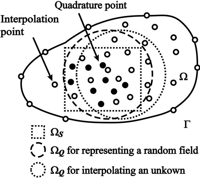
Figure 1. Difference between WS and WQ.
ishes, this equation contains no domain integrals. Therefore, if Equation (5) is adopted to derive a spectral stochastic meshless local Petrov-Galerkin formulation, computing the resulting spectral stochastic meshless local Petrov-Galerkin formulation is more time-saving than computing the published spectral stochastic meshless local Petrov-Galerkin formulation [5].
Moreover, substituting
 into Equation (5) yields
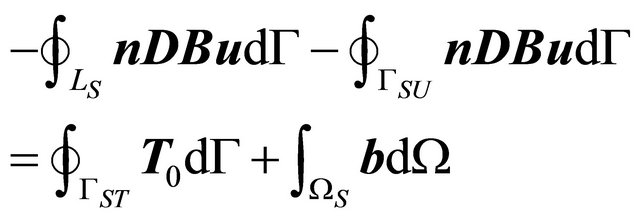 (6)
(6)
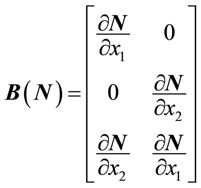
where l is the Lamè constant, G is the shear modulus, u = [u1, u2]T,  , b = [b1, b2]T, and
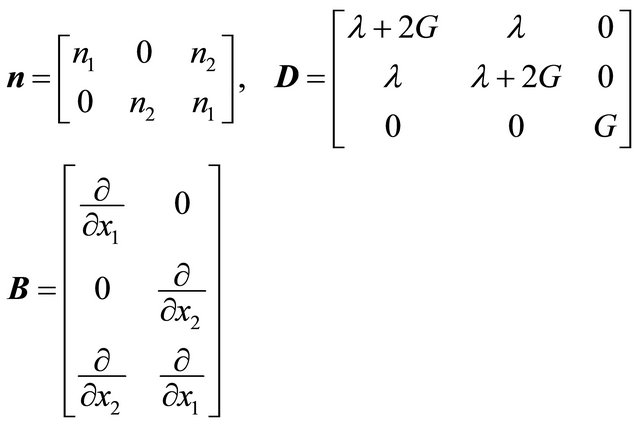 (7)
(7)
Next, similarly manipulating a published radial basis function-based interpolation formula [5], u over WQ for a node is approximated by
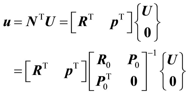 (8)
(8)
where ,
,  , M is the total number of nodes within an WQ, the subscript i is the i-th node,
  ,
,
 is a complete monomial basis of order m, Ri, i = 1 to M represent the radial basis function, and
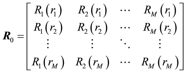 (9a)
(9a)
 (9b)
(9b)
in which x1 to xM represent those M nodes within WQ for xI, and ri to rM represents the Euclidean distance between xI and each node within WQ for xI. Constructing N for further details can be seen in the published study [5].
Substituting Equation (8) into Equation (6) and writing the resulting expressions more succinctly in matrix algebra yield
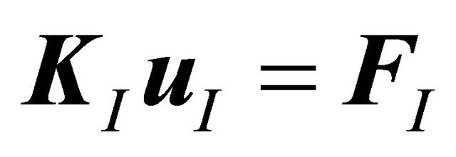 (10)
(10)
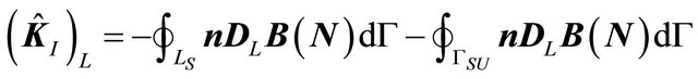
where K and F are; respectively, the stiffness and force matrices, the subscript I represents the contribution to K or F at xI (I = 1 to NT), 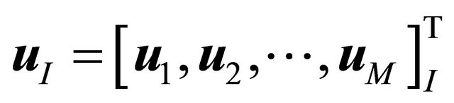 , KI and FI are derived by
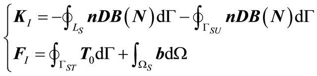 (11)
(11)
where the subscripts i and j denote i-th and j-th node within WQ for xI (I = 1 to NT); respectively and
 (12)
(12)
Repeatedly deriving Equation (10) for all NT nodes and assembling all the resulting expressions based on a global numbering system yield
 (13)
(13)
Since this study accounts for the uncertainty in the spatial variability of mechanical properties in predicting the structural failure probability pf, the generalized polynomial chaos expansion is introduced to represent random mechanical properties. The next section presents the relevant derivation.
3. Spectral Stochastic Meshless Local Petrov-Galerkin Formulation
Observing the derivation of Equation (13) needs mechanical properties G and l. Thus, the generalized polynomial chaos expansions of G and l are [5]
 (14)
(14)
where , Yi represent the multivariate orthogonal polynomial of x,
  denote multi-dimensional uncorrelated random variables having zero mean and unit variance (for facilitating the computation of mean values and standard deviations of G and l), NPC is equal to (n + P)!/n!P!–1, P is the highest order of Y, and n is the total number of uncorrelated random variables.
For facilitating the construction of Equation (14), Y0, Ĝ0, and  are; respectively, set to 1, mG, and ml in which mG, and ml are mean values of G and l; respectively. Furthermore, computing Ĝi, and
  (i = 1 to NPC) needs the orthogonal relationship,
  (i, j = 0 to NPC) in which
 ![]() is the ensemble average. For example, Ĝi (i = 0 to NPC) are computed by
is the ensemble average. For example, Ĝi (i = 0 to NPC) are computed by
 (15)
(15)
where ![]() is computed as follows: If f and g are two functions,
is computed as follows: If f and g are two functions, ![]() is computed by 1) Continuous case:
is computed by 1) Continuous case:
 (16a)
(16a)
2) Discrete case:
 (16b)
(16b)
where  are the weighting functions. Since the succeeding study focuses on the continuous random fields, Table 1 [6] lists examples of orthogonal polynomials, statistical distributions and weighting functions to generate Yi (i = 0 to ¥),
  , and
, and ; respectively.
Substituting Equation (14) into Equation (11) yields
 (17)
(17)
in which DL represents the computation of D using ĜL and (L = 0 to M) and
 (18)
(18)
Since the expressions of FI doesn’t contain G and l, substituting the generalized polynomial chaos expansions
Table 1. Examples of polynomials and corresponding weighting functions and statistical distributions for generating the generalized polynomial chaos [6].

Note that [a, b] denotes a specific interval.
of G and l into FI is unnecessary. Meanwhile, the generalized polynomial chaos expansion of u is
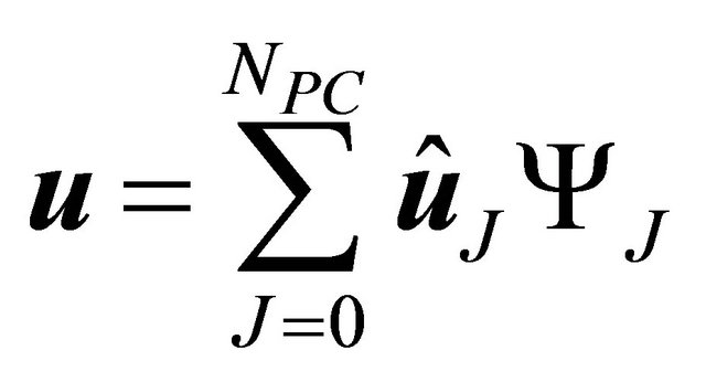 (19)
(19)
Substituting Equations (17) and (19) into Equation (11) results in
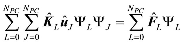 (20)
(20)
Requiring the residual resulting from a finite representation of u (i.e. truncating ûJYJ,  ) to be orthogonal to the approximation space spanned by YJ yields
 (21)
(21)
in which k = 0 to NPC. Solving Equation (21) can obtain ûJ (J = 0 to NPC). Collecting the resulting ûJ can construct the generalized polynomial chaos expansion of u.
4. First Order Reliability Method
This study introduces structural reliability assessment problems to evaluate the performance of Equation (21). Estimating this structural reliability follows the firstorder reliability method [9]; therefore, this section summarizes the first-order reliability method.
Given a traction T0 bearing on a structure subjected to the uncertainty in the spatial variability of G and l, a vector X having components G and l at all NT nodes is created. In addition, a performance state function g(X) is defined to identify the failure (g(X) < 0) and safe states (g(X) > 0) of the structure. For example, a book [11] emphasizes T0 and its resistance R; thus, g(X) is
 (22)
(22)
Moreover, a space of different X values is plotted and the location of g(X) is marked. Figure 2 [12] illustrates the special case of X = (X1, X2). In this figure, suppose the point A denotes the point  and the structure is safe at this point. Observing Figure 2 can know that the shortest distance between point A and g(X) sizes the range of X values within which a safe structural design is expected. Extending this observation, the shortest distance between
  and g(X) sizes the range of X values within which a safe structural design is expected. Hasofer and Lind (1974) [9] defined the shortest distance between
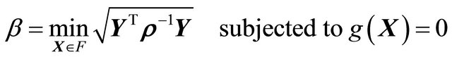
  and g(X), in units of directional standard deviations as the reliability index b. They concluded that searching b is a constrained optimization problem in the form as [12]
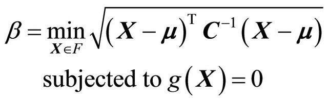 (23)
(23)
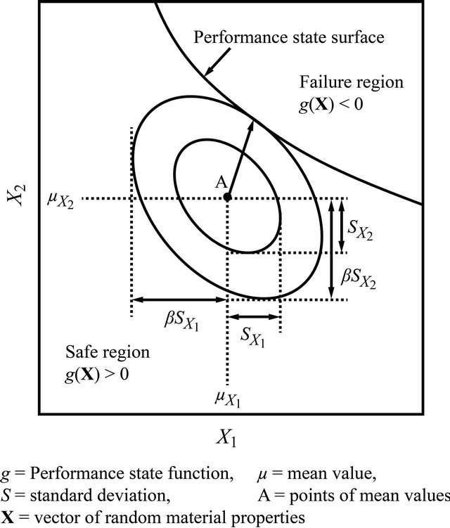
Figure 2. Search of the reliability index b [12].
where F denotes the failure region on the space of X,  , and C is the covariance matrix.
A number of algorithms have been developed to solve Equation (23) or similar equations. This study chooses a popular algorithm suggested by Lowe and Tang [12]. Briefly, this algorithm is based on the Rackwitz-Fiessler equivalent normal transformation [13] but the concepts of coordinate transformation and frame-of-reference rotation are not applied. Correlation is accounted for by setting up the quadratic form directly. Similarly manipulating the previous study [12], three steps are performed to solve Equation (23):
1) Modify Equation (23) with standard normal random variables. Transform the vector X into a new vector of Y having standard normal random variables Yi (i = 1 to 2NT) in the form as
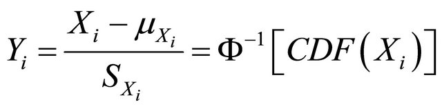 (24)
(24)
in which 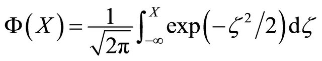 is the cumulative probability function of a standard normal distribution, CDF is the cumulative probability function computed at Xi. Using the new vector Y, Equation (23) is modified to
 (25)
(25)
in which r is the correlation matrix evaluated at Y.
2) Start from Yi = 0 (i = 1 to 2NT) (or ) to search the X value causing g(X) = 0. In searching such an X value, increase Y values and calculate the corresponding X value by Table 2 [12]. Note that this table is edited
Table 2. Obtaining Xi from Yi based on CDF(Xi) = F(Yi) [12].
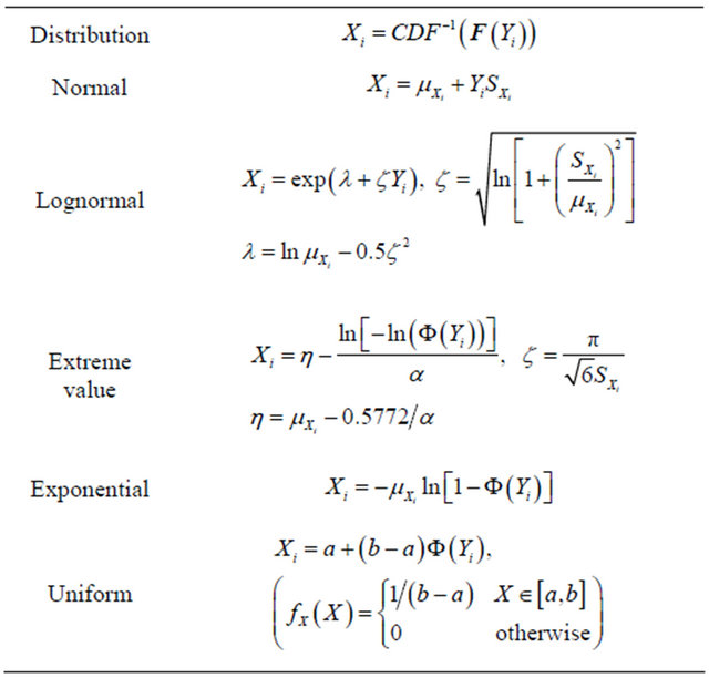
fX = probability density function.
by choosing those probability distributions, which may be applied in the current study.
3) To incorporate with a spectral stochastic meshless local Petrov-Galerkin FORTRAN code, a VA10AD subroutine [14] is introduced to automate the above two steps.
After finding the X value causing g(X) = 0 and computing the corresponding b value from Equation (25), the structural failure probability pf is estimated by
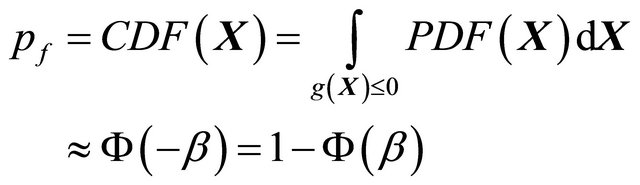 (26)
(26)
where PDF is the probability density function.
5. Results and Discussions
Two benchmark problems are introduced to evaluate the performance of Equation (21). As a comparison, the spectral stochastic finite element method is applied to the same problems. The FERUM package [15] is adopted to generate spectral stochastic finite element results. The first benchmark problem involves bending of a cantilever beam by a parabolically distributed traction at its free end. The second benchmark problem involves bending of a dam caused by the fluid pressure. Except for inspecting the accuracy of spectral stochastic meshless local Petrov-Galerkin-based predicted pf, two different radial basis functions are; respectively, adopted to construct N in solving those two problems; thus, the effects of different radial basis functions on the accuracy of spectral stochastic meshless local Petrov-Galerkin results can be observed.
5.1. Bending of a Cantilever Beam by a Parabolically Distributed Traction
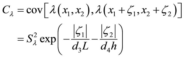
Suppose the cantilever beam has the length L, width h, and unit thickness. Figure 3 illustrates the layout of this cantilever beam and boundary conditions in which Q denotes the integration of parabolically distributed traction along the x2 direction and the point B is subsequently used to define the performance state function g(X). If any uncertainty is neglected, the analytical solution of u2 is [10]
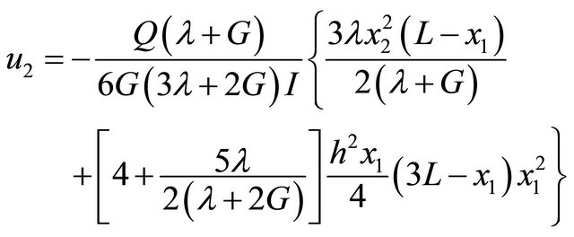 (27)
(27)
where I = h3/12 is the moment of inertia and Q is integration of the parabolically distributed traction along the x2 direction. Since only the analytical solution of u2 is adopted subsequently to implement the Monte Carlo simulation, analytical solutions of u1 and sij (i, j = 1 to 2) are not listed here. Interested readers can find these analytical solutions in the book [10].
Nevertheless, this study accounts for the uncertainty in random G and l in predicting pf. Assume G and l vary according to
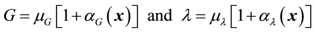 (28)
(28)
where aG and al are two homogeneous Gaussian random fields with zero mean and having the following covariance functions CG and Cl:
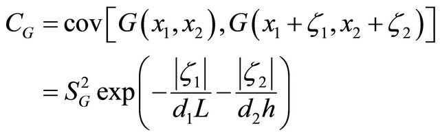 (29a)
(29a)
 (29b)
(29b)
in which cov represents the covariance, (x1, x2) and (x1 +
Figure 3. Bending of a cantilever beam by a parabolically distributed at its ends (not to scale, i = 1 to 2).
z1, x2 + z2) are two points on the cantilever beam, SG and Sl are; respectively, standard deviations of G and l, and di (i = 1 to 4) are four correlation parameters.
To predict pf of the cantilever beam with the uncertainty in random G and l, essential data are listed below 1) Define the problem domain W as 0 £ x1 £ L and –h/2 £ x2 £ h/2.
2) Generate two cases of meshless discretizations and one case of finite element discretization. Figure 4 illustrates these meshless (top and middle sub-figures) and finite element discretizations (bottom sub-figure) in which the meshless discretization of randomly located nodes (middle sub-figure) is obtained by randomly distributing the meshless discretization of equally spaced nodes (bottom sub-figure).
3) Experiment to represent G, l, and u by the Lauguerre polynomial chaos.
4) Set a complete monomial basis pT = [1, x1, x2] (m = 3). Setting such a low-order of p is intentional. Observing the accuracy of corresponding numerical results is desired.
5) Construct N by the Gaussian radial basis function; that is, 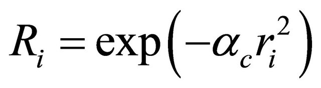 (i = 1 to M) where ac (³ 0) is a shape parameter.
6) Choose each WQ as a circle centered at a point and each WS as a rectangular centered at a node. The length and width of each WS and radius of each WQ are set subsequently.
7) Define the performance state function g(X) by
 (30)
(30)
where ud is a threshold of displacement and the subscript B denotes the point B in Figure 3.
8) Generate Monte Carlo simulation results to serve as the accuracy standard in comparing spectral stochastic finite element-based and spectral stochastic meshless local Petrov-Galerkin-based predicted pf. Following a book [11] the first step of implementing a Monte Carlo simulation is sampling of G and l according to Equation (28). Each sample of G and l are then substituted into
Figure 4. Meshless and finite element discretizations for analyzing the first benchmark problem.
Equation (27) to compute a sample of u2,B. If Nsample is the total number of samples of u2,B and N(g(X) £ 0) is the total number of samples of u2,B causing the structural failure, pf is computed by
 (31)
(31)
Moreover, the resulting pf can be inverted to compute the reliability index b. If G and l are sufficiently sampled, the Monte Carlo simulation-based pf and b approach their exact values.
9) Unless otherwise stated, the following parameters are adopted: L = 48 m, h = 12 m, NPC = 10, mG = 11.5 MPa, ml = 17.3 MPa, ac = 0.03, Hs = 9.6 m, BS = 6 m, rQ = 6 m, Nsample = 106, Nq = 16, di = 1 (i = 1 to 4), Q = 103 kN where HS and BS are; respectively, the height and width of each WS, rQ is the radius of each WQ, and Nq is the total number of quadrature points in each WS or finite element.
Moreover, in order to state quantitatively the accuracy of spectral stochastic meshless local Petrov-Galerkin or spectral stochastic finite element results, two error estimators D and d are defined below
 (32)
(32)
in which the subscripts MCS, SSMLPG, and SSFEM denote the Monte Carlo simulation, spectral stochastic meshless local Petrov-Galerkin and spectral stochastic finite element methods; respectively.
Figure 5 compares variation of the predicted PDF of u2 at the point B versus different prediction methods
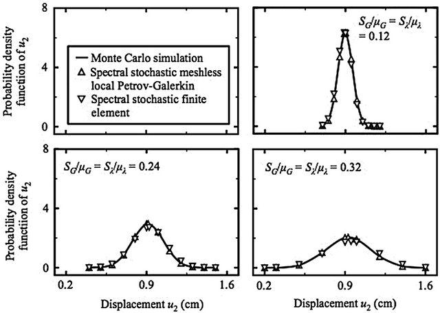
Figure 5. Variation of the predicted probability density function of u2 at the point B versus different SG/mG and Sl/ml values (First benchmark problem, meshless discretization: the top sub-figure of Figure 4, d1 = d2 = d3 = d4 = 1).
and SG/mG = Sl/ml = 0.12, 0.24, 0.32. Figure 6 (in the next page) presents variation of the predicted pf at the point B versus different ud values, prediction methods, and SG/mG = Sl/ml = 0.12, 0.24, 0.32. Furthermore, Table 3 compares the time spent to produce the spectral stochastic meshless local Petrov-Galerkin-based and Monte Carlo simulation-based predicted pf with SG/mG = Sl/ml = 0.12.
Benefiting from adopting the MLPG5 scheme to derive a spectral stochastic meshless local Petrov-Galerkin formulation, Table 3 indicates that generating spectral stochastic meshless local Petrov-Galerkin results is considerably time-saving, even if the Monte Carlo simulation is implemented using analytical solutions. Meanwhile, Figure 5 illustrates the necessity of predicting u with the uncertainty in the spatial variability of G and l. When the SG/mG and Sl/ml values increase, the standard deviation of u2 increase; thus, obtaining the predicted u2, which is different from its mean value, becomes more and more possible. In addition, Figure 6 presents that the spectral stochastic meshless local Petrov-Galerkin method predicts more accurate pf than the spectral stochastic finite element method does. For example, if computing D and d values with SG/mG = Sl/ml = 0.12, the resulting D value approximately peaks at 0.36 %; whereas, the resulting d value peaks about at 13.97 %.
Nevertheless, the performance of both Equation (21)
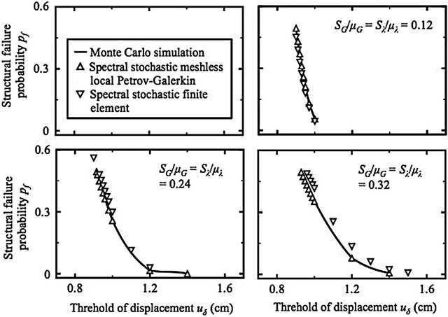
Figure 6. Variation of the predicted structural failure probability pf at the point B versus different SG/mG and Sl/ml values (first benchmark problem, meshless discretization: the top sub-figure of Figure 4, d1 = d2 = d3 = d4 = 1).
Table 3. Comparison of the time spent to generate Monte Carlo simulation and spectral stochastic meshless local Petrov-Galerkin results*.
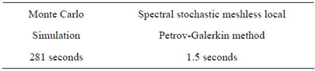
*On a MacBook Pro with an Intel Core i5 Processor, GFortran compiler.
and spectral stochastic finite element method becomes gradually unsatisfactory when SG/mG and Sl/ml increases. If SG/mG and Sl/ml values measure the degree of uncertainty, Figure 6 outlines that the degree of uncertainty can apparently reduce the accuracy of predicted u or pf. Furthermore, observing Equations (29a) to (29b) can find that decreasing di (i = 1 to 4) values and increasing SG/mG and Sl/ml values have similar effects on the accuracy of predicted u or pf.
Next, replacing Lauguerre polynomial chaos with Hermite polynomial chaos to represent G, l, and u, Figure 7 compares spectral stochastic meshless local Petrov-Galerkin-based predicted pf values versus different types of the polynomial chaos, SG/mG = Sl/ml = 0.12, and different ud values.
Figure 7 implies the importance of preparing some pilot tests before choosing a specific type of polynomial chaos to represent a random field. Calculating D values using this figure finds that the performance of Lauguerre polynomial chaos is more satisfactory. If G and l are represented using the Hermite polynomial chaos, the corresponding D value peaks at about 2.758%.
Next, replacing meshless discretization of equally spaced nodes (the top sub-figure of Figure 4) with meshless discretization of randomly located nodes (the middle sub-figure of Figure 4), Figure 7 re-compares variation of Monte Carlo simulation-based and spectral stochastic meshless local Petrov-Galerkin-based predicted pf values versus different ud values, and SG/mG = Sl/ml = 0.12.
Computing the D value using data in Figure 8 finds that the resulting D value peaks at about 2.367%. Consequently, Equation (21) still predicts pf sufficiently accurately, even if a meshless distribution of discrete nodes is adopted. Moreover, in an attempt of more understanding the effects of different nodal spacings on the accu-
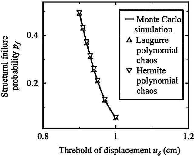
Figure 7. Variation of the predicted structural failure probability pf at the point B versus different types of the polynomial chaos (first benchmark problem, meshless discretization: the upper sub-figure of Figure 4, d1 = d2 = d3 = d4 = 1).
racy of predicted pf, the problem domain W is re-discretized using equally spaced nodes and NT = 27 (3 ´ 9), 52 (4 ´ 13), 85 (5 ´ 17). Figure 9 depicts the corresponding variation of Monte Carlo simulation-based and spectral stochastic meshless local Petrov-Galerkin-based predicted pf versus different h values, ud = 0.95 cm, and SG/mG = Sl/ml = 0.12 where h denotes the spacing of any two connecting nodes.
Figure 9 reports that the effects of different h values on the accuracy of predicted pf are not noticeable. For example, if the NT value increases from 52 (3 ´ 9) to 85 (5 ´ 17), the corresponding D value only changes slightly; consequently, adopting more nodes for improving the accuracy of Monte Carlo simulation-based or spectral stochastic meshless local Petrov-Galerkin-based predicted pf is laborious.
5.2. Bending of a Dam Caused by Fluid Pressure
Suppose the dam has the length L, width h, and unit thick-
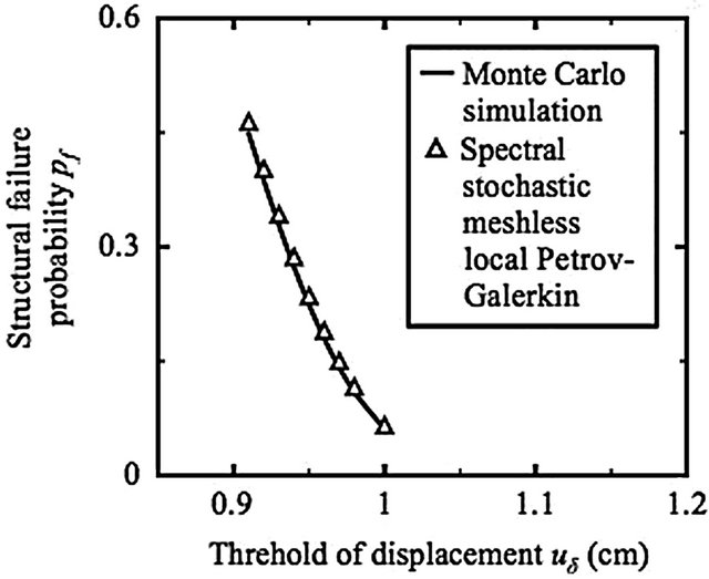
Figure 8. Variation of the predicted structural failure probability pf at the point B versus randomly nodal distribution (first benchmark problem, meshless discretization: the middle sub-figure of Figure 4, d1 = d2 = d3 = d4 = 1).
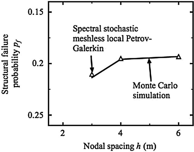
Figure 9. Variation of the predicted structural failure probability pf at the point B versus different nodal spacing h (m) (First benchmark problem, meshless discretization: the upper sub-figure of Figure 4, d1 = d2 = d3 = d4 = 1).
ness. This dam is fixed at one end and subjected to fluid pressure. Figure 10 illustrates the layout of problem domain W and boundary conditions in which C and D are subsequently used to define the performance state function and gf is the unit weight of fluid.
If any uncertainty is neglected, the analytical solutions of u1 and u2 are [10]
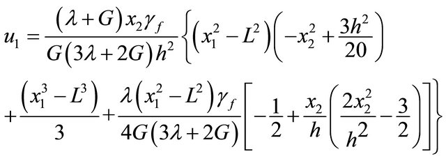 (33a)
(33a)
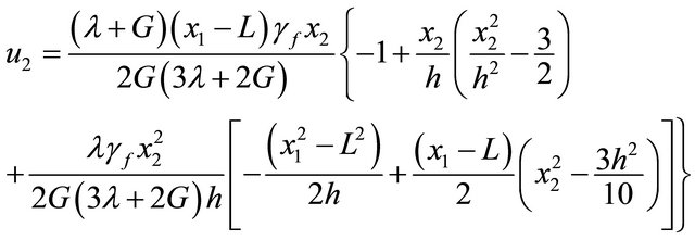 (33b)
(33b)
However, suppose G and l vary according to two uniform distributions:
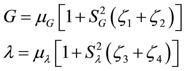 (34)
(34)
where –1 < zi (i = 1 to 4) < 1 represent four random variables.
To predict pf of the dam with the uncertainty in random G and l, the essential data are provided below:
1) Define the problem domain W as –h/2 £ x2 £ h/2 and 0 £ x1 £ L.
2) Generate a meshless discretization and a finite element discretization. Figure 11 presents these meshless
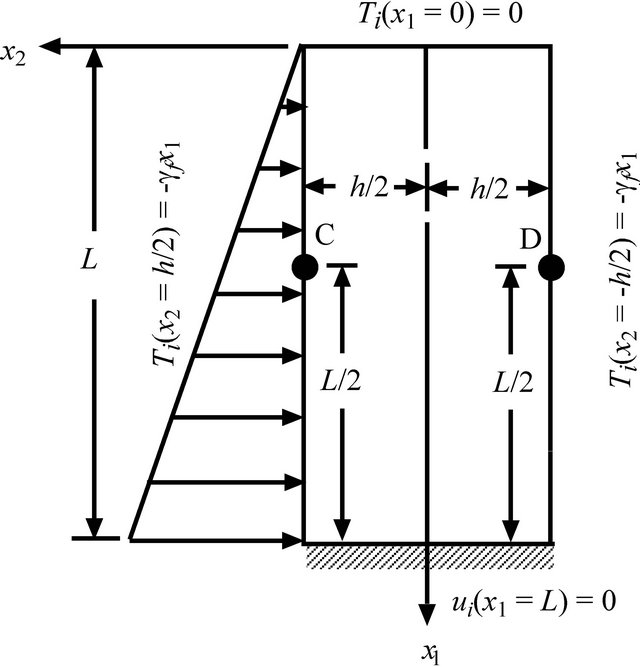
Figure 10. Bending of a dam caused by fluid pressure [10] (not to scale, i = 1 to 2).
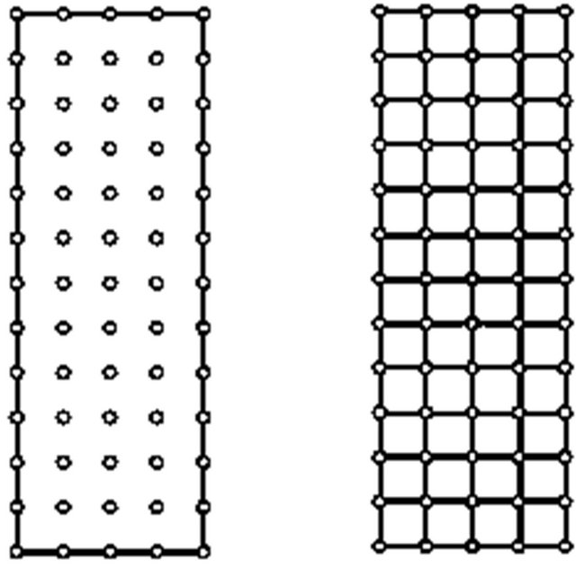
Figure 11. Meshless and finite element discretizations for analyzing the second benchmark problem.
and finite element discretizations.
3) Represent G, l, and ui (i = 1 to 2) by the Legendre polynomial chaos.
4) Still set a complete monomial basis pT = [1, x1, x2] but adopt the multiquadric radial basis function to construct f; that is, 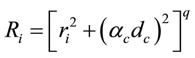 (i = 1 to M) where ac (³0) and q are two shape parameters and dc is the characteristic length related to the nodal spacing in an WQ.
5) Define two performance state functions g1(X) and g2(X) as follows:
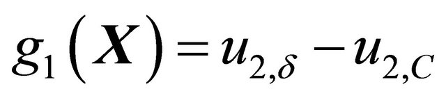 (35a)
(35a)
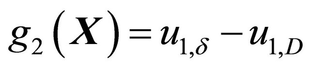 (35b)
(35b)
where ui,d (i = 1 to 2) are two thresholds of displacements and the subscripts C and D denote the points C and D in Figure 10.
6) Similarly manipulate point (8) in Section 5.1 but replace Equation (27) with Equations (33a) to (33b) to generate the Monte Carlo simulation-based predicted pf. The resulting Monte Carlo simulation-based predicted pf serves as the accuracy standard in comparing the spectral stochastic meshless local Petrov-Galerkin and spectral stochastic finite element results.
7) Unless otherwise stated, the following data are used: L = 30 m, h = 10 m, gf = 9.81 kN/m3, NPC = 10, mG = 11.5 MPa, ml = 17.3 MPa, ac = 1.0, dc = 3.0, q = 1.03, HS = 5 m, BS = 5 m, rQ = 5 m, Nsample = 106, and Nq = 16.
Figure 12 (in the next page) compares variation of the pf at the point C with respect to SG/mG = Sl/ml = 0.12, 0.24, 0.32, different prediction methods and u2,d values. Figure 13 (in the next page) compares variation of the pf at the point D with respect to SG/mG = Sl/ml = 0.12, 0.24, 0.32, different prediction methods and u1,d values.
Observing Figure 12 confirms that the performance of
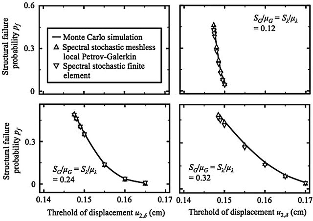
Figure 12. Variation of the predicted structural failure probability pf at the point C versus different SG/mG and Sl/ml values (Second benchmark problem).
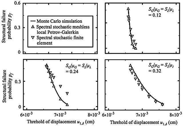
Figure 13. Variation of the predicted structural failure probability pf at the point D versus different SG/mG and Sl/ml values (Second benchmark problem).
spectral stochastic meshless local Petrov-Galerkin method is more satisfactory than the performance of spectral stochastic finite element method. Even if different statistical distributions are encountered, Figures 6, 12, and 13 present the spectral stochastic meshless local PetrovGalerkin results are more accurate than the spectral stochastic finite element results. In addition, careful inspection of spectral stochastic finite element results in Figures 12 to 13 finds that the errors between Monte Carlo simulation and spectral stochastic finite element results majorly source from inaccurate spectral stochastic finite element-based predicted mean values of u at the points C and D. Resolving this problem may need high-order finite elements. But, to the author’s knowledge, similar experiences seem to be seldom seen.
6. Conclusions
Prior to the previous [5] and current studies, available stochastic numerical methods include the Monte Carlo simulation, spectral stochastic finite element, and stochastic element-free Galerkin methods. The Monte Carlo simulation is simplest. As demonstrated in Sections 5.1 and 5.2, implementing the Monte Carlo simulation only needs deterministic solutions. Even so, as outlined by Table 3, completing the Monte Carlo simulation is still more time-consuming than generating the spectral stochastic meshless local Petrov-Galerkin results. Producing such results attributes to that the total number of samples for implementing a Monte Carlo simulation is usually very large.
Meanwhile, applying the spectral stochastic finite element method is easy, since numerous resources (computer software and experiences) are available. Nevertheless, based on these resources, this study finds that the spectral stochastic finite element results of some problems are less accurate than spectral stochastic meshless local Petrov-Galerkin results of the same problems. Sections 5.1 and 5.2 provide two examples.
Together with the previous study [5], the succeeding study provides a new alternative for solving stochastic boundary-value problems. This new stochastic numerical method is truly-meshless. As demonstrated in Sections 5.1 and 5.2, no finite elements or background cells for the numerical integration are created in applying the spectral stochastic meshless local Petrov-Galerkin method. However, the spectral stochastic meshless local PetrovGalerkin method successfully spend less time but still predict the accurate structural failure probability pf in Sections 5.1 and 5.2.
In conclusion, the spectral stochastic meshless local Petrov-Galerkin method is a time-saving tool for solving stochastic boundary-value problems.
REFERENCES
- R. G. Ghanem and P. D. Spanos, “Stochastic Finite Elements: A Spectral Approach,” Revised Edition, Dover Publications, New York, 2012.
- S. Rahman and B. N. Rao, “An Element-Free Galerkin Method for Probabilistic Mechanics and Reliability,” International Journal of Solids and Structures, Vol. 38, No. 50-51, 2001, pp. 9313-9330.
- V. Papadolous, G. Soimiris and M. Papadrakis, “Buckling Analysis of I-Section Portal with Stochastic Imperfections,” Engineering Structures, Vol. 47, 2013, pp. 54-66. doi:10.1016/j.engstruct.2012.09.009
- K. Sepahvand, S. Marburg and H.-J. Hardtke, “Stochastic Free Vibration of Orthotropic Plates Using Generalized Polynomial Chaos Expansion,” Journal of Sound and Vibration, Vol. 331, No. 1, 2012, pp. 167-179. doi:10.1016/j.jsv.2011.08.012
- G. Y. Sheu, “Prediction of Probabilistic Settlements via Spectral Stochastic Meshless Local Petrov-Galerkin Method,” Computers and Geotechnics, Vol. 38, No. 4, 2011, pp. 407-415. doi:10.1016/j.compgeo.2011.02.001
- D. Xiu and G. E. Karniadakis, “Modeling Uncertainty in Flow Simulations via Generalized Polynomial Chaos,” Journal of Computational Physics, Vol. 187, No. 1, 2003, pp. 137-167. doi:10.1016/S0021-9991(03)00092-5
- S. N. Atluri and T. Zhu, “A New Meshless Local PetrovGalerkin (MLPG) Approach in Computational Mechanics,” Computational Mechanics, Vol. 22, No. 2, 1998, pp. 117-127. doi:10.1007/s004660050346
- S. N. Atluri and S. Shen, “The Meshless Local PetrovGalerkin (MLPG) Method,” Tech Science Press, Ecino, 2002.
- A. M. Hasofer and N. C. Lind, “Exact and Invariant Second-Moment Code Format,” Journal of Engineering Mechanics ASCE, Vol. 100, No. 1, 1974, pp. 1227-1238.
- S. Timoshenko and J. N. H. Goodier, “Theory of Elasticity,” 3rd Edition, McGraw-Hill Publishing Company, New York, 1970.
- R. E. Melchers, “Structural Reliability Analysis and Prediction,” 2nd Edition, John Wiley and Sons, England, 1999.
- B. K. Low and W. H. Tang, “Efficient Spreadsheet Algorithm for First-Order Reliability Method,” Journal of Engineering Mechanics ASCE, Vol. 133, No. 12, 2007, pp. 1378-1387. doi:10.1061/(ASCE)0733-9399(2007)133:12(1378)
- R. Rackwitz and B. Fiessler, “Structural Reliability under Combined Random Load Sequences,” Computers and Structures, Vol. 9, No. 5, 1978, pp. 484-494. doi:10.1016/0045-7949(78)90046-9
- R. Fletcher, “VA10AD Harwell Subroutine Library,” A. E. R. E. Harwell, Oxfordshire, 1972.
- B. Sudret and A. D. Kiureghian, “Stochastic Finite Elements and Reliability: A State-of-Art Report,” Report No. UCB/SEMM-2000/08, University of California, Berkeley, 2000.