World Journal of Mechanics
Vol.2 No.4(2012), Article ID:21535,9 pages DOI:10.4236/wjm.2012.24023
Interactive Visualization System of Taylor Vortex Flow Using Stokes’ Stream Function
Department of Mechanical Engineering, Meijo University, Nagoya, Japan
Email: furukawa@meijo-u.ac.jp
Received May 2, 2012; revised June 9, 2012; accepted June 18, 2012
Keywords: Taylor Vortex Flow; Axisymmetric Flow; Interactive Visualization System; Computational Fluid Dynamics; Fluid Informatics
ABSTRACT
Taylor vortex flow between two concentric rotating cylinders with finite axial length includes various patterns of laminar and turbulent flows, and its behavior has attracted great interests. When mode bifurcation occurs, quantitative parameters such as the volume-averaged energy change rapidly. It is important to visualize the behaviors of vortices. In this study, a three-dimensional visualization system with respect to time is devised. This system can change the viewpoint of flow visualization, and we can observe the track of a vortex from any point. The volume-averaged energy is projected to the track of the center of a vortex. The proposed system can help to investigate the relationship between the mode bifurcation process and the volume-averaged energy.
1. Introduction
Taylor vortex flow has been studied as an important vortex flow since it was first reported by Taylor in 1923 [1]. In a concentric double cylinder, when the rotation speed of the inner cylinder is gradually increased from zero, Couette flow first occurs in the gap between the inner and outer cylinders. When the rotation speed of the inner cylinder is further increased, Couette flow changes to Taylor vortex flow, in which many torus flows called cells are stacked, then to wavy Taylor vortex flow, and finally to turbulent flow. Taylor vortex flow often appears in journal bearings, hydrodynamic machines and containers for chemical reactions, and clarification of the mechanism of Taylor vortex flow is highly important for the engineering field.
Since Taylor’s study, Taylor vortex flow has been studied by many researchers, and the complexity of the flow has been clarified. Unsteady flow (e.g. Taylor vortex flow) causes unstable change in the physical quantities that characterize the flow. Pacheco et al. [2] showed experimentally that in small aspect-ratio Taylor-Couette flows have a band in the parameter space where rotating waves become steady nonaxisymmetric solutions via infinite-period bifurcations. Martinand et al. [3] showed that imposing axial flow in the annulus and radial flow through the cylindrical walls in a Taylor Couette system alters the stability of the flow. To analyze these unsteady flows, authors focused on quantitative values such as a mean energy [4]. The kinetic energy and enstrophy for flows with different final modes are compared.
In this study, the flow structure of Taylor vortex flow is investigated numerically, where the inner cylinder is rotating, and the outer cylinder and both the upper and lower end walls are stationary. The main parameters in this study are the aspect ratio which is the ratio of the cylinder length to the gap between the cylinders, and the Reynolds number, which is estimated from the velocity of the inner cylinder. Changes in these parameters lead to the generation of various flow structures. In this study, the mode formation process and the bifurcation of Taylor vortex flow are analyzed.
2. Identification of Vortices
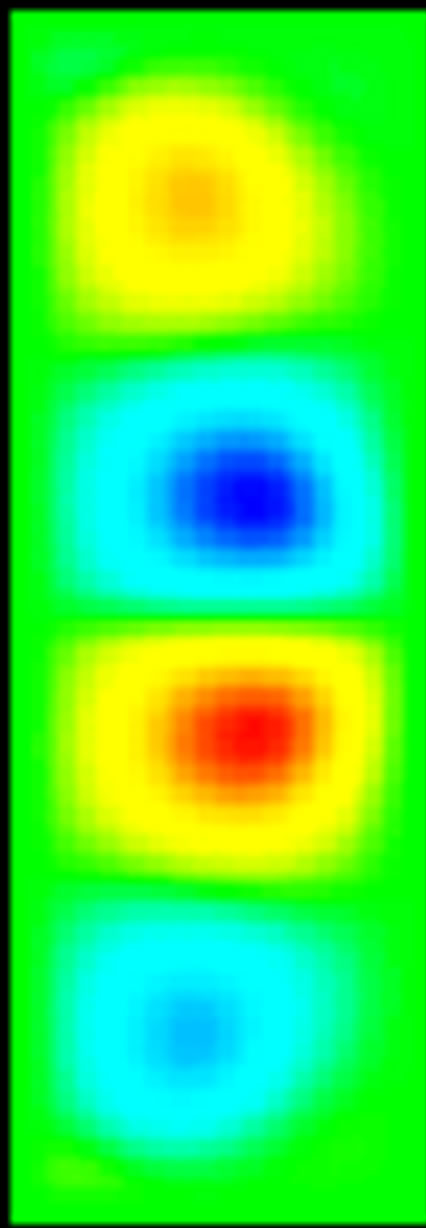
The most common method of identifying vortices is to use the velocity vector (Figure 1(a)). Figures 1(b)-(d) show the visualization methods using the vorticity, Q invariant and Stokes’ stream function, respectively. The visualization method using vorticity cannot distinguish the vortices. The center positions obtained using the Q invariant do not correspond to the centers of the vortices. On the other hand, the center positions obtained using Stokes’ stream function shows good agreement with those obtained from the velocity vector.
Figure 2 shows a comparison between the velocity vector and Stokes’ stream function. The left-hand figure is a schematic flow pattern of the normal four-cell mode
 (a)
(a)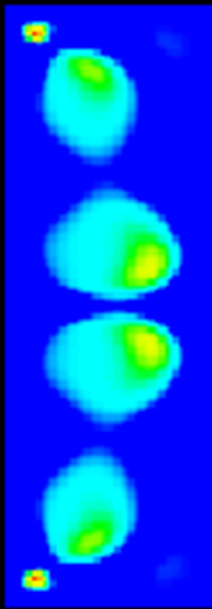 (b)
(b)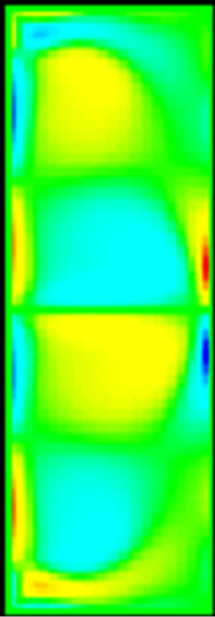 (c)
(c)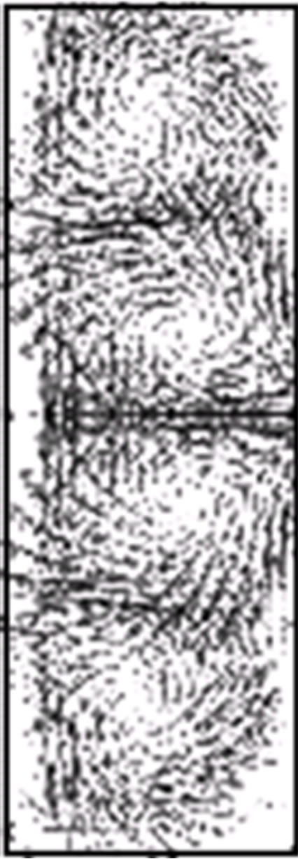 (d)
(d)
Figure 1. Comparison of visualization methods. (a) Velocity vector; (b) Vorticity; (c) Q invariant; (d) Stream function.
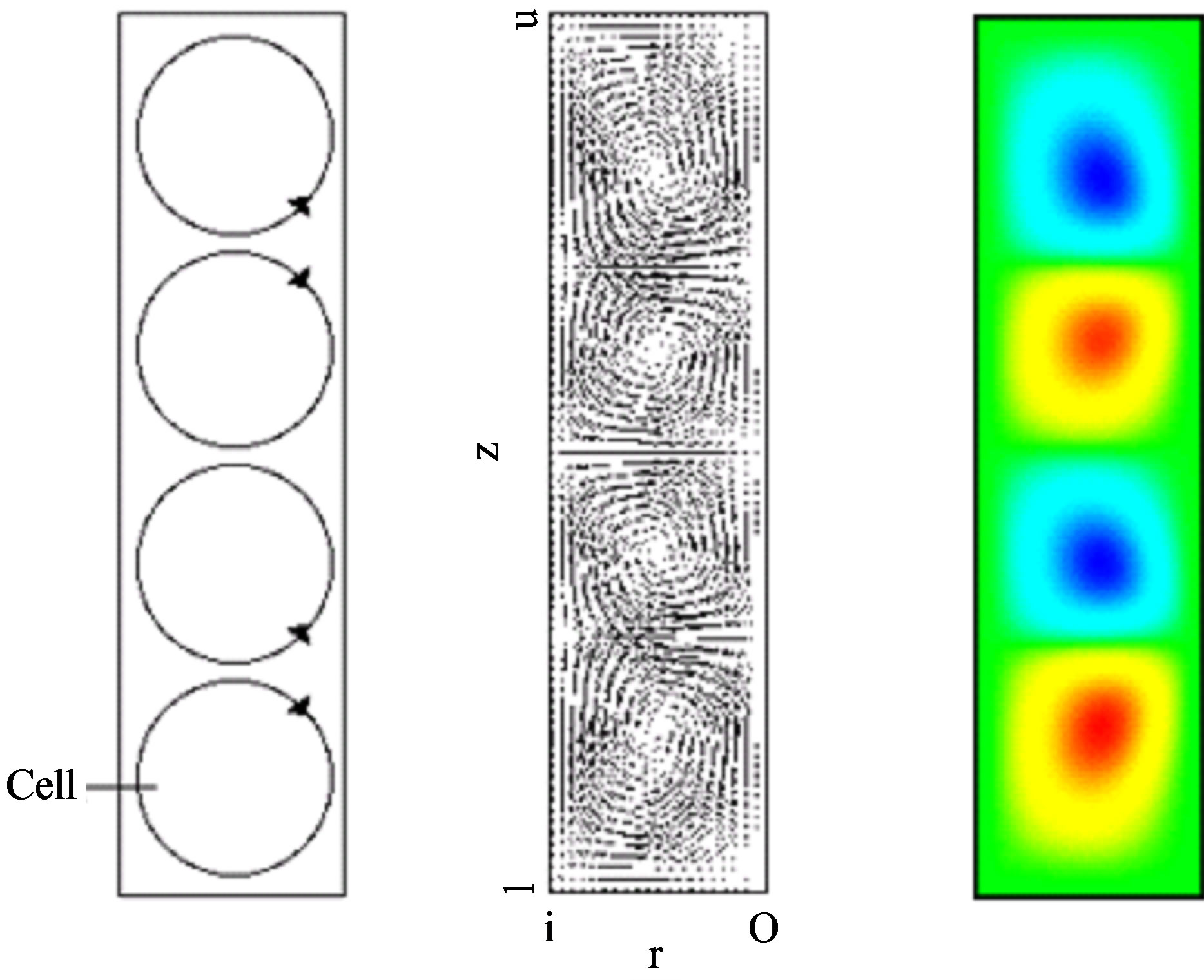
Figure 2. Comparison for N4.
(N4). The center figure and right-hand figure respecttively show the velocity vector and the contours of Stokes’ stream function. The contours of Stokes’ stream function can be clearly used to identify the centers of vortices. Moreover, using Stokes’ stream function it is possible to distinguish the borders of vortices. Figure 3 shows the flow of the anomalous four-cell mode (A4). Stokes’ stream function can be used to confirm the existence of extra vortices and to identify the centers of the extra vortices. Thus, the contours of Stokes’ stream function are adopted to analyze the mode formation process and the bifurcation of Taylor vortex flow in this study.
3. Numerical Method
The governing equations are the axisymmetric unsteady incompressible Navier-Stokes equation with cylindrical coordinates (r, θ, z) and the continuity equation.
We use both SOR and ILUCGS methods to solve Poisson’s equation for pressure. The stress-free boundary
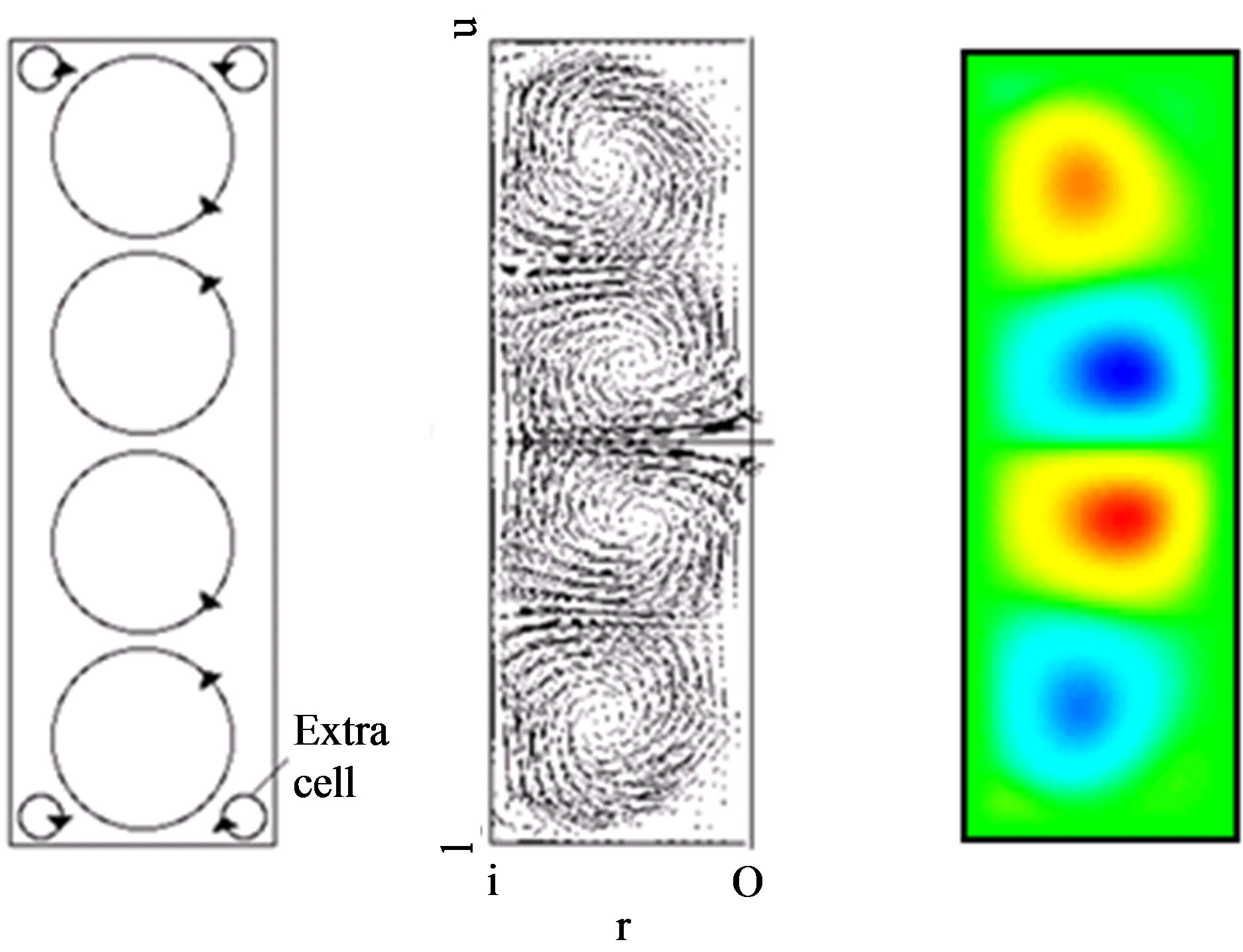
Figure 3. Comparison for A4.
condition was used for the upper end wall and the stationary (non-slip) condition is used for the lower end wall. We applied Neumann conditions based on the momentum equation for pressure. As the initial condition, all velocity components are zero. Mixed solution of water and glycerin is assumed to be the working fluid, and its dynamic viscosity is 6.0 × 10⁻⁶ m2/s. For the discretization method, we apply the QUICK method for convection terms, the second-order central difference method for the other space integration, and Euler’s method for the time integration. Grids are staggered and equidistant in each direction. The number of grid points is 41 in the radial direction, and the number of grid points in the axial direction is proportionally adjusted so that it becomes approximately 42 for the aspect ratio of 1.0. In order to examine the validity of the number of grid points, we analyzed Taylor vortex flow using several types of grids under various numerical conditions, and concluded that there are no differences among the modes that are finally formed, the formation of modes up to the final mode, and the manner of decay of the vortexes.
4. Method of Tracking Unsteady Motion
Figure 4 shows Taylor vortex flow. The right hand figure shows the contours of Stokes’ stream function ψ, defined as follows.
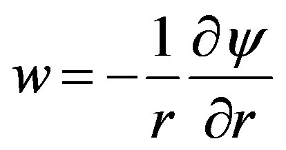
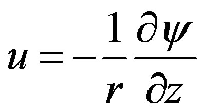 (1)
(1)
Here, u and w are the velocity components in the radial and circumferential direction, respectively, and r denotes the coordinate in the radial direction. In Figure 4, the left hand indicates the rotating inner cylinder and the right hand shows the stationary outer cylinder. The red region indicates where ψ becomes positive, that is, the cell is rotating clockwise. The blue region indicates where ψ is negative, that is, and the cell rotating counterclockwise.
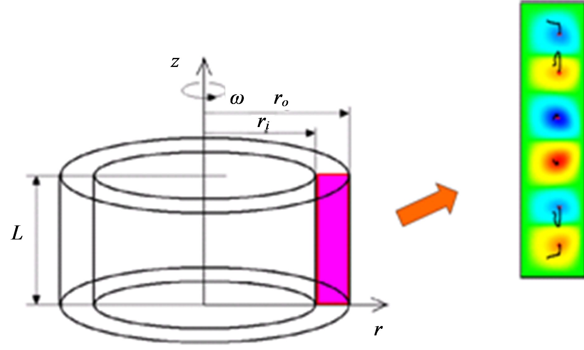
Figure 4. Taylor vortex flow.
There are extreme in the contours of the stream function. The positions of which the extreme values of the stream function appear are defined as the centers of vortices. The black lines in Figure 4 are the trajectories of the centers of vortices. The centers are important parameters for showing the flow structure.
The modes of Taylor vortex flow are roughly divided into two: normal modes and anomalous modes. The normal and anomalous modes are defined as below and depend on the end-wall boundary condition of the cylinder and the flow direction in the vicinity of the end walls. When the cylinder end wall is stationary, the normal mode has a flow from the outer cylinder to the inner cylinder (inward flow) in the vicinity of the end wall, while the anomalous mode has a flow from the inner cylinder to the outer cylinder (outward flow). In the previous study, it was confirmed that the anomalous mode has extra vortices [5].
The following variables are defined: the radii of the inner and outer cylinders are ri and ro, respectively, and the radius ratio η ( ri/ro) is set to 0.667. The aspect ratio Γ is the ratio of the cylinder length, L, to the radial difference between the cylinders, D (= ro – ri). The angular velocity of the inner cylinder is ω, and the Reynolds number, Re, is estimated using ri, ω and D. All physical parameters are made dimensionless using the characteristic length L and characteristic velocity riω.
5. Correspondence of Vortices
It is necessary to confirm that the history of each center completely corresponds. When the past and current centers of vortices are identical, it is called complete correspondence. When they are different, it is called noncorrespondence. Incomplete correspondence is defined as a flow in which the past and current vortices belong to same vortex but do not appear to be identical. The conditions used to classify the correspondence of vortices are as follows:
1) The distance between the past and current centers of a vortex is less than 5 lattices.
2) The past and current centers of a vortex are included in the same vortex.
Complete correspondence satisfies both 1) and 2), noncorrespondence does not satisfy both 1) and 2), and incomplete correspondence is defined as other than these cases.
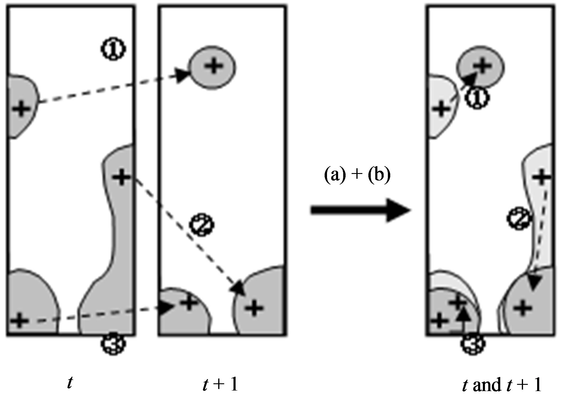
Figure 5(a) shows a flow field at time step t, and Figure 5(b) shows the flow field at time step t + 1. Figure 5(c) shows a comparison of the vortices and their centers between time step t and t + 1. Plus signs denote the centers. The arrows and numbers show the correspondence of the history of each vortex. Number 1 shows an example of noncorrespondence. The center of the vortex at time step t is not included in the area of the vortex at time step t + 1. Moreover, the center of the vortex at time step t + 1 is not included in the area of the vortex at time step t. Number 2 shows an example of incomplete corresponddence. Although the centers of the vortex at time steps t and t + 1 are included in the same vortex area, the distance between the centers at time steps t and t + 1 is more than 5 lattices. Number 3 shows an example of complete correspondence. The centers of the vortex at time steps t and t + 1 are included in the same vortex area, and the distance between centers of the vortices is less than 5 lattices.
6. Tracking of Vortex Behavior
6.1. Flow Development of Normal Mode
Figure 6 shows tracks illustrating the formation process of the normal two-cell mode (N2). The Reynolds number is 200, and the aspect ratio is 3.0 in this calculation model. Vortices develop near the center of the inner cylinder at the fixed wall, and a total of six unstable vortices develop, including the two produced at the upper and lower ends of the cylinder. The vortices at the upper and
 (a) (b) (c)
Figure 5. Pattern diagrams showing process of tracking vortices.
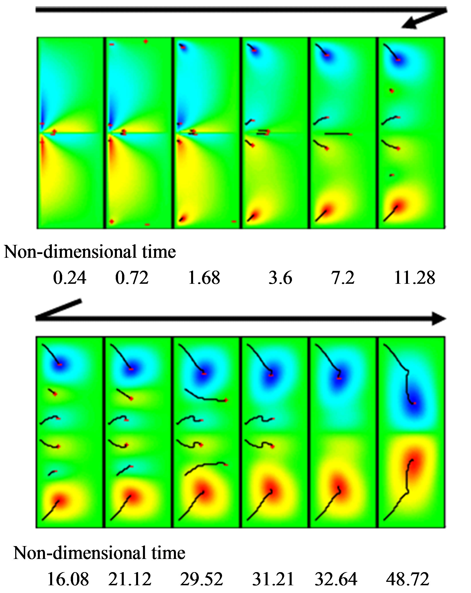
Figure 6. Flow development of N2. (Re: 200, Γ: 3.0).
lower ends remain, and where the four central vortices are absorbed and eventually disappear. The two remaining vortices become stable, and the normal two-cell mode develops. The figure clearly shows that the visualization system in this study successfully captures the tracks of the centers of the vortices.
6.2. Flow Development of Anomalous Mode
Figure 7 shows the mode formation process of the anomalous four-cell mode (A4). The Reynolds number is 650, and the aspect ratio is 4.2. First, vortices are produced near the center of the inner cylinder, and then they grow. Other vortices are produced at the ends of the inner cylinder. The transition of the mode to the anomalous four-cell mode begins when the nondimensional time is about 31.2. Four extra vortices are observed near both upper and lower end walls.
7. Three-Dimensional Display Using Java3D
In the previous analysis, we presented the calculated results in two dimensions. However, to investigate the time dependence of the mode formation process, it is necessary to present the position of each vortex with respect to time. To clarify the complex process of vortex development with respect to time, we represent the behaviors of vortices in three dimensions using the Java3D library. Figure 8 shows an example of a track of a vortex obtained using the interactive visualization system. The calculation step axis is shown in green, the radial direction is in yellow and the axial direction in blue. In this
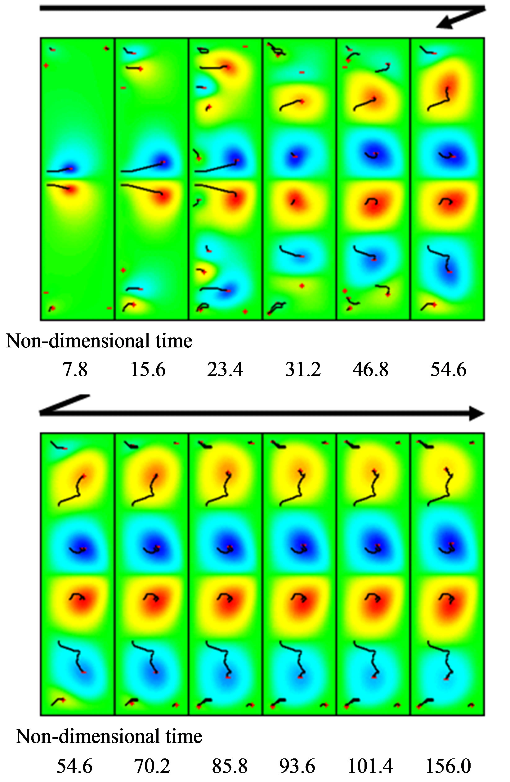
Figure 7. Flow development of A4. (Re: 650, Γ: 4.2).
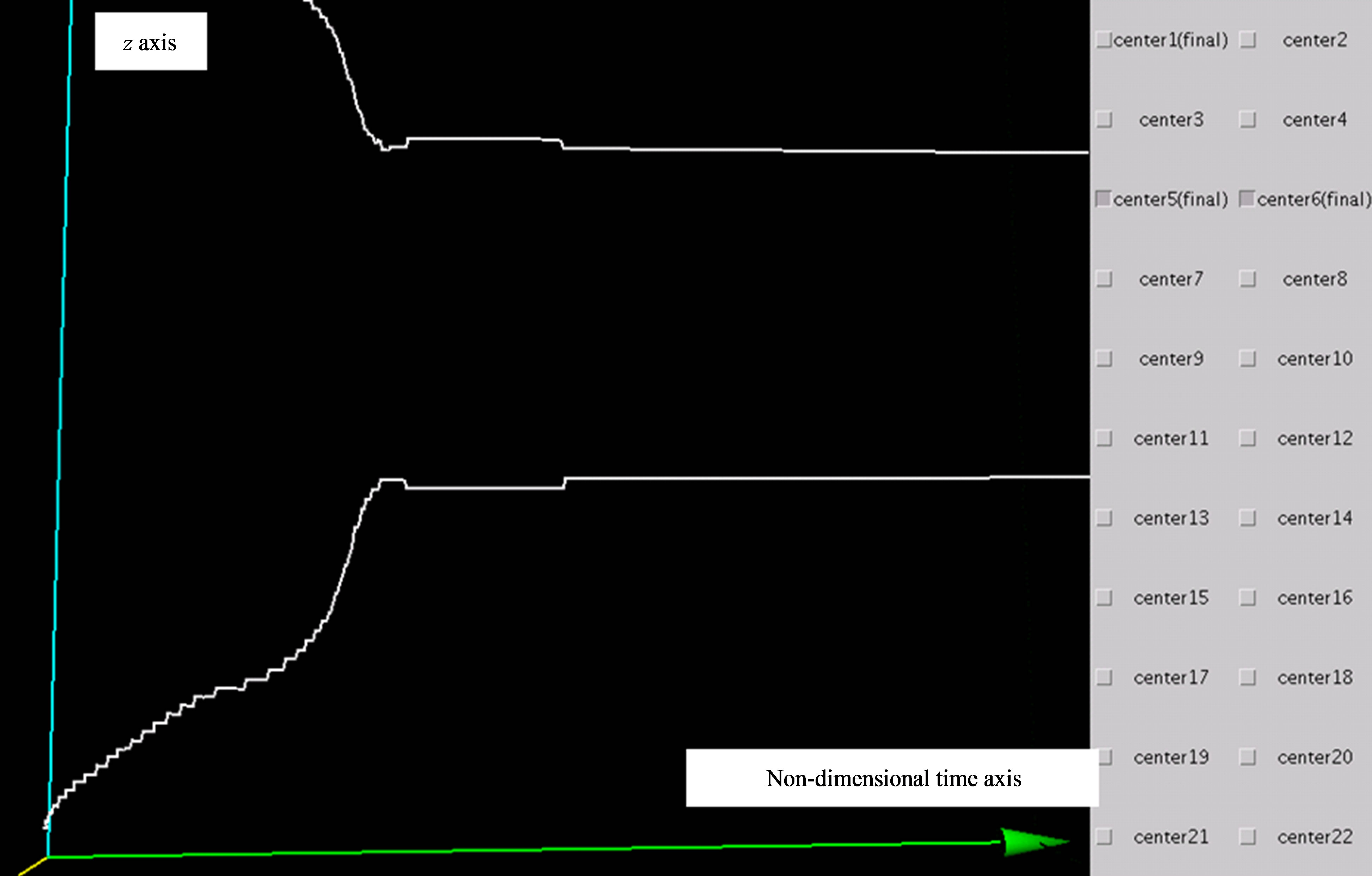
system, the viewpoint of flow visualization can be changed. (Figure 9) We can observe the track of a vortex from any point by dragging the mouse, or by keyboard operation. The number attached to each box shown on the right-hand side of the screen corresponds to the number assigned to the center of the vortex. Only the tracks of the centers of vortices whose boxes have a check mark are displayed. The tracks of multiple centers can be displayed by checking multiple boxes. When a vortex remains until the final mode, the word “final” is added to the end of the center number after the check box.
Such vortices play an important role in mode formation processes.
Three-Dimensional Display of Normal Mode
Figure 10 shows the tracks of a vortex that remained until the final normal two-cell mode. The Reynolds number of 200, and an aspect ratio of 3.0 are used, which are the same as the conditions used for Figure 6. Figure 10 shows calculated results using the Java3D library for the t-z plane observed from the r direction and for the r-z plane observed from the direction of the calculation time step axis. Two vortices that develop at the upper and lower ends of the inner cylinder gradually move to the middle of the cylinder in the vertical direction and remain of a constant distance. They then move horizontally.
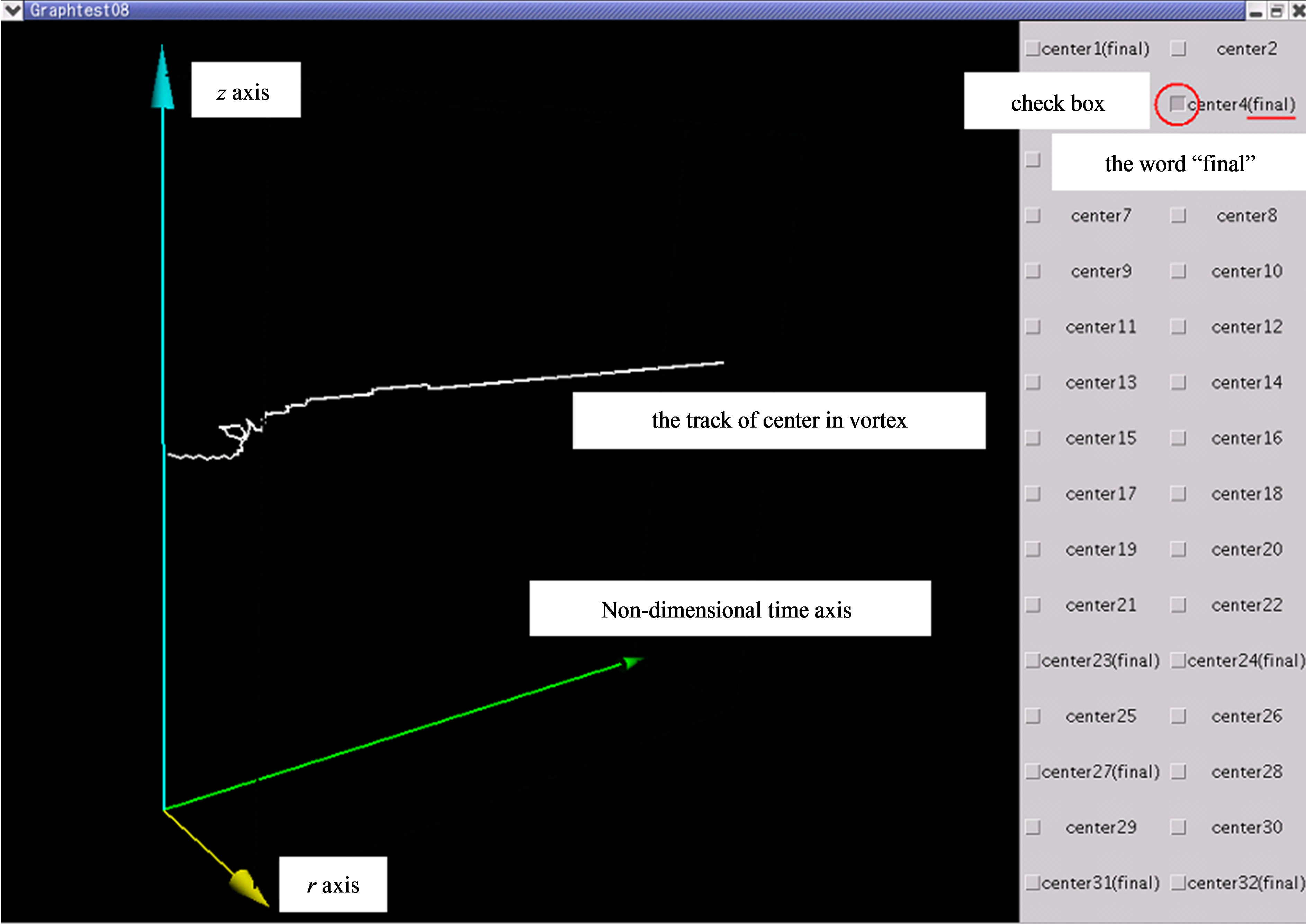
Figure 8. 3D visualization system.
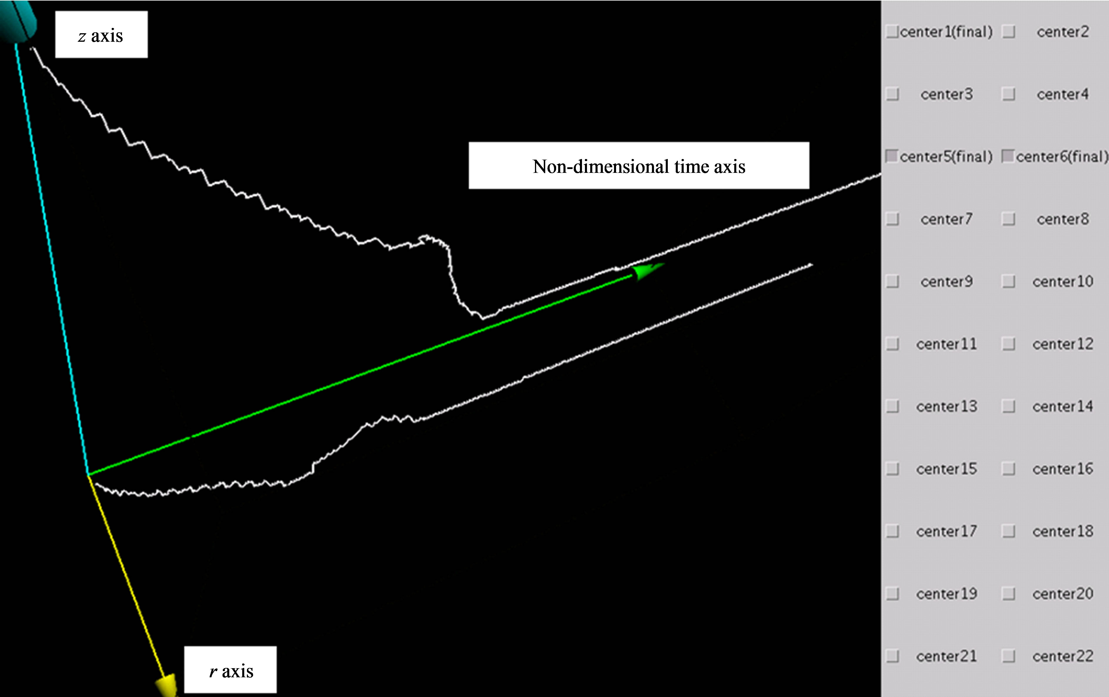
Figure 9. Example of 3D display.
 (a)
(a)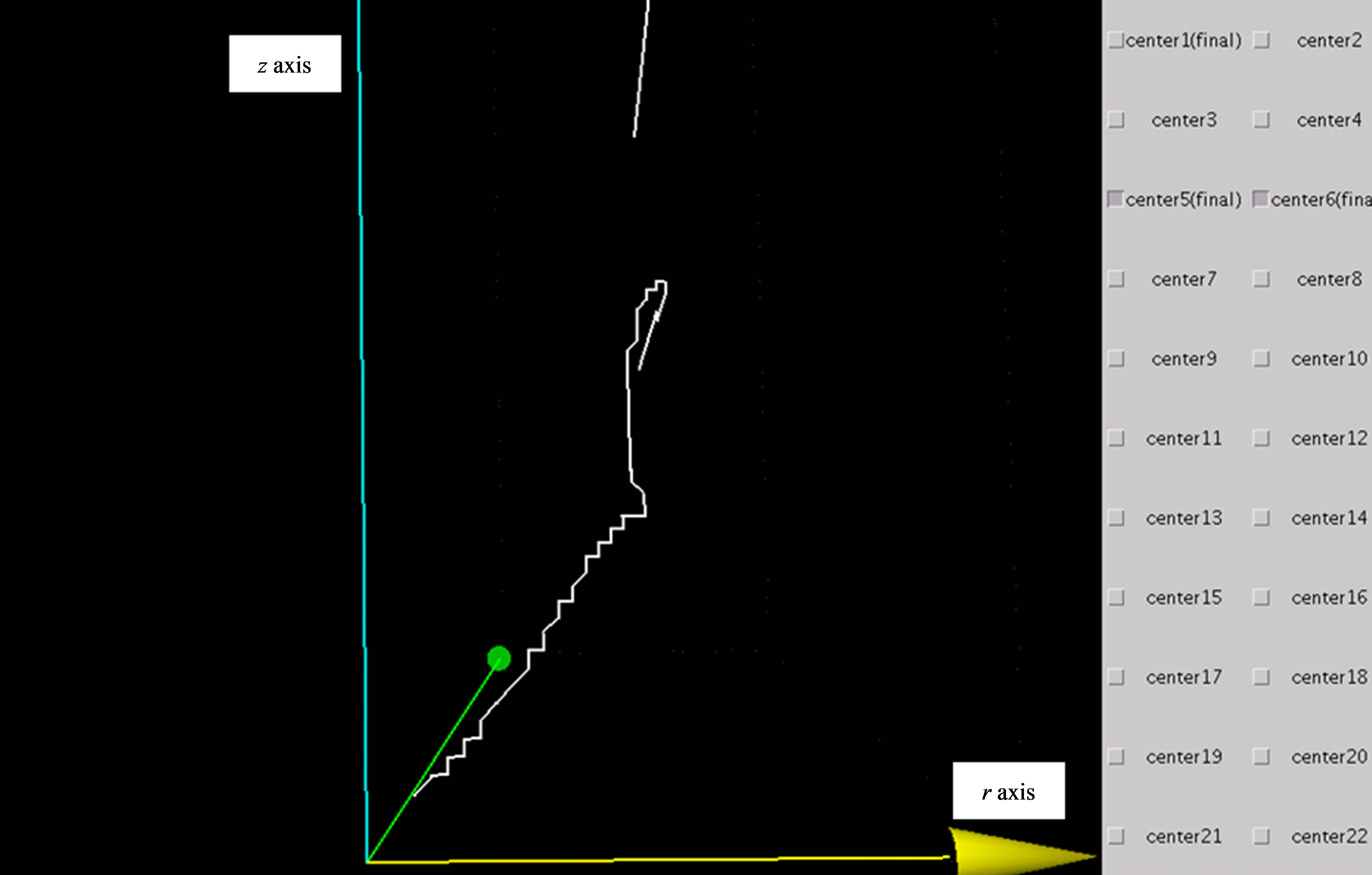 (b)
(b)
Figure 10. Example of 3D display. (Re: 200, Γ: 3.0). (a) Nondimensional time-z plane; (b) r-z plane.
The centers of the two vortices move symmetrically with respect to the midplane in the axial direction.
8. Projection of Quantitative Parameter
8.1. Bifurcation Process of Taylor Vortex Flow
When the Reynolds number is changed after a stable mode appears, a mode bifurcation occurs and the flow becomes another mode. Figure 11 shows the tracks of vortex centers during the formation process from the normal four-cell mode to the normal two-cell mode. A change in the Reynolds number is from 700 to 350, and an aspect ratio is 2.8. The Reynolds number is kept constant up to a nondimensional time of 2100, and then it is decreased linearly from 700 to 350 at nondimensional time of 4200. The Reynolds number is 700 in the figures showing Stokes’ stream function contours 1 to 7, and is decreased from 700 to 350 in the figures showing Stokes’ stream function contours 8 to 11. The Reynolds number is 350 in the figure showing Stokes’ stream function contours 12. In the bifurcation process, two centers vortices are initially larger than the upper and lower vortices until the figure showing Stokes’ stream function contour 4. The upper and lower vortices gradually develop, and each vortex begins to oscillate after a nondimensional
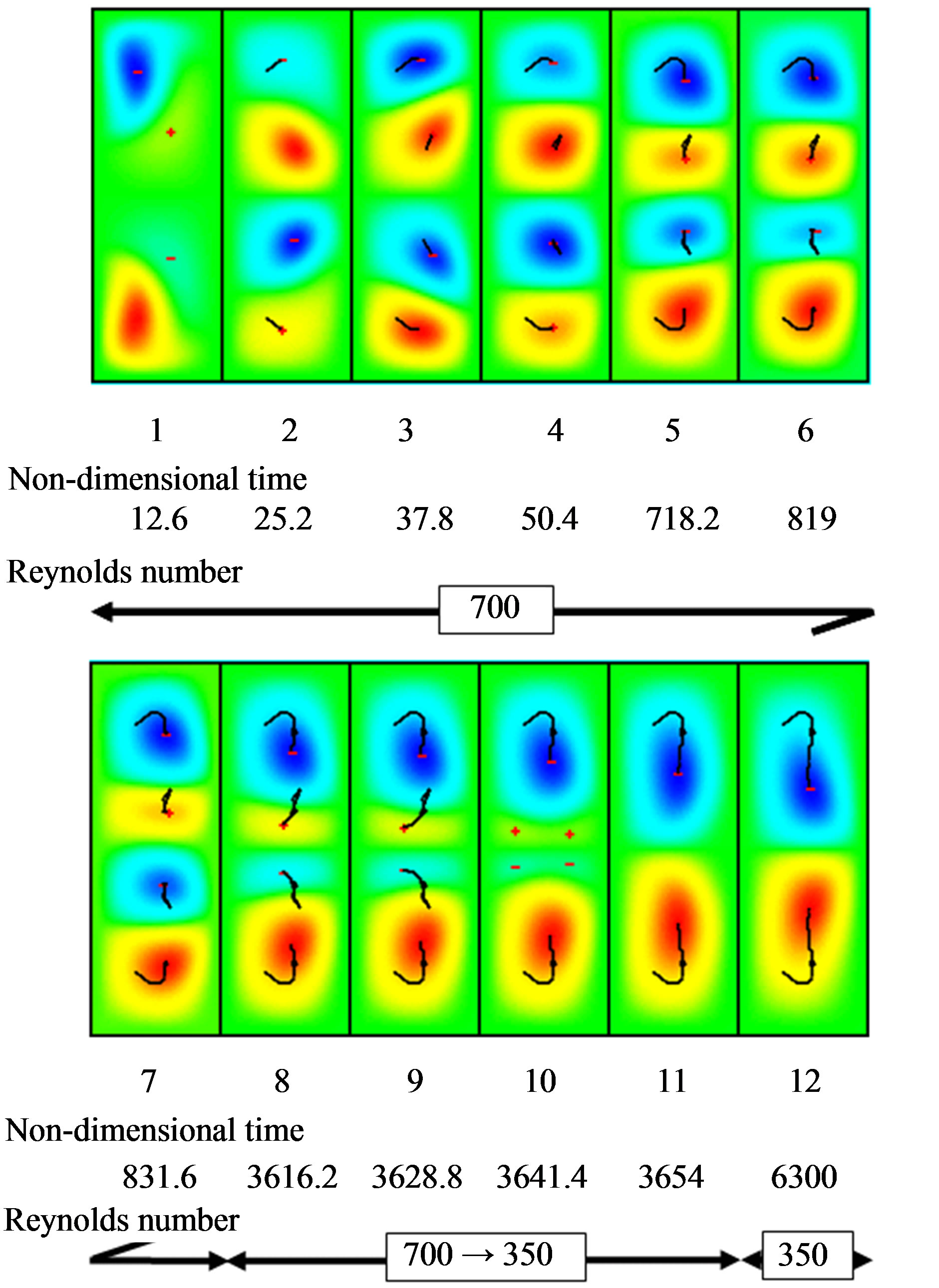
Figure 11. Mode formation process from N4 to N2. (Re: 700 - 350, Γ: 2.8).
time of 600. After the Reynolds number begins to decrease, the pair of vortices near the midplane in the axial direction become smaller. The two center vortices weaken and disappear, and finally the flow becomes the normal two-cell mode.
8.2. Bifurcation Process Displayed in Three Dimension
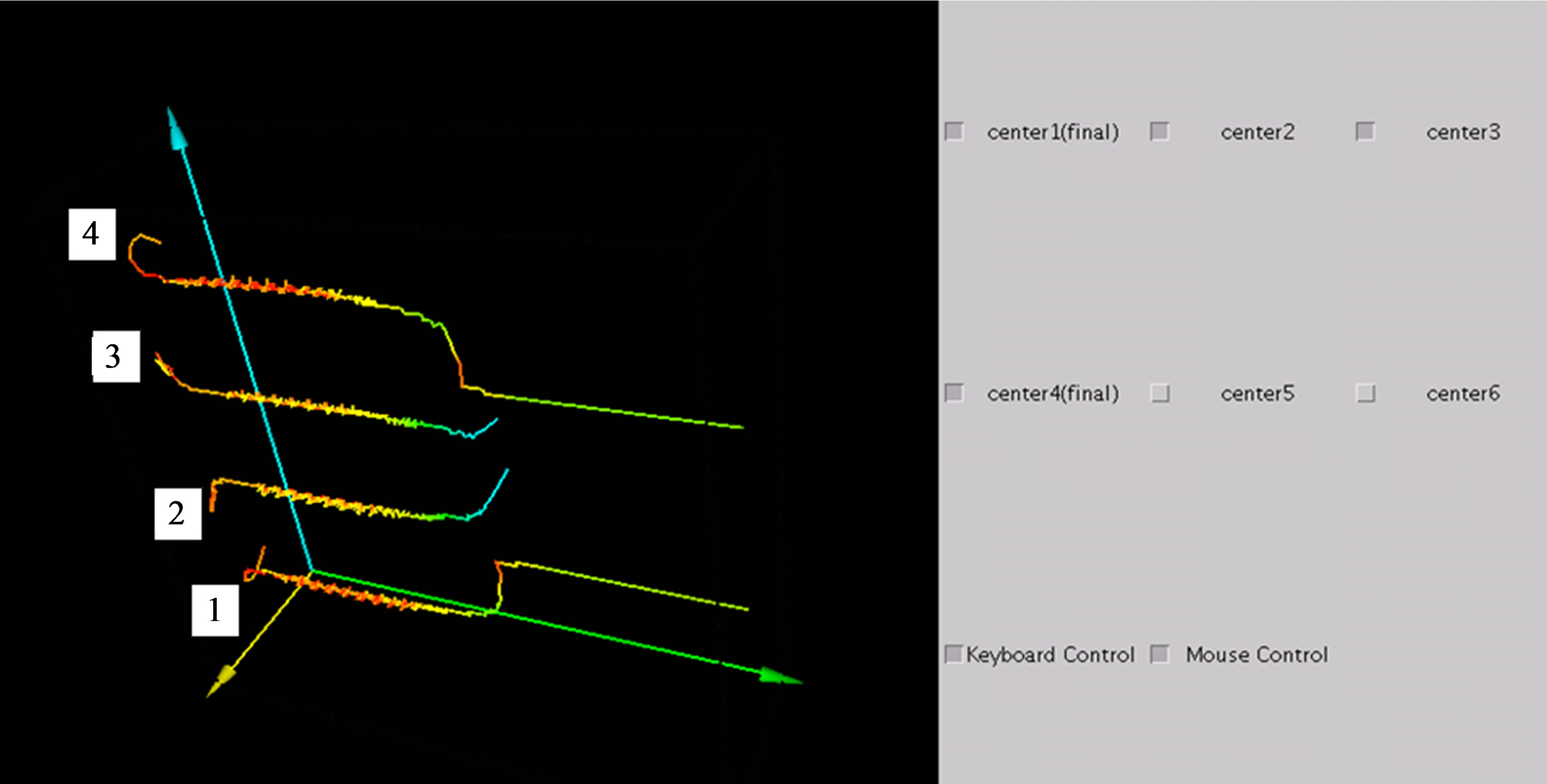
During the mode bifurcation, the characteristic parameters such as the volume-averaged energy oscillate and affect the flow structure. In this study, we develop an interactive visualization system that can project the quantitative parameter of each vortex to the track line in three dimensions. Figure 12 shows the tracks of vortices obtained using the interactive visualization system. The Reynolds number and aspect ratio are the same as those in Figure 11. The color of each track indicates the volume-averaged energy. High values are shown in red, and low values are shown in blue. Using this method, we can clarify the relation between the flow behavior and volume-averaged energy.
The tracks of the centers of the vortices numbered by 1 - 4 are shown in Figure 12(a). Regions A and B are shown in Figure 12(b). Region A includes time steps 5 - 7 shown in Figure 11, while region B contains time steps 8 - 11. The positions of the centers oscillate slightly in region A. In this region, the change in color indicates the oscillation of the volume-averaged energy in vortices 1 and 4. After the decrease in the Reynolds number, the oscillation disappears. Comparing each vortex, the volume-averaged energies of vortices 1 and 4 are higher than those of vortices 2 and 3 when the Reynolds number is 700. After the decrease in the Reynolds number, vortices 2 and 3, whose volume-averaged energies are low, weaken and disappear. Then, the remaining vortices become stable and the normal two-cell mode appears. This mode transition occurs during the time shown in region B. After vortices 2 and 3 disappear, the volume-averaged energies of vortices 1 and 4 become high. After that, the volume-averaged energies of the remaining vortices decrease and the flow field becomes stable.
9. Discussion
To display the tracking results in three-dimensions, we followed the centers of the vortices using the Java3D library. Using this method, we can observe the mode formation processes in three-dimensional coordinates. Tracks showing the movement of vortices before their full development and vortices with complicated behavior that are difficult to observe by a two-dimensional representation can easily be observed. Observation of the development process from various viewpoints is an effective means of tracking the development of vortices.
 (a)
(a)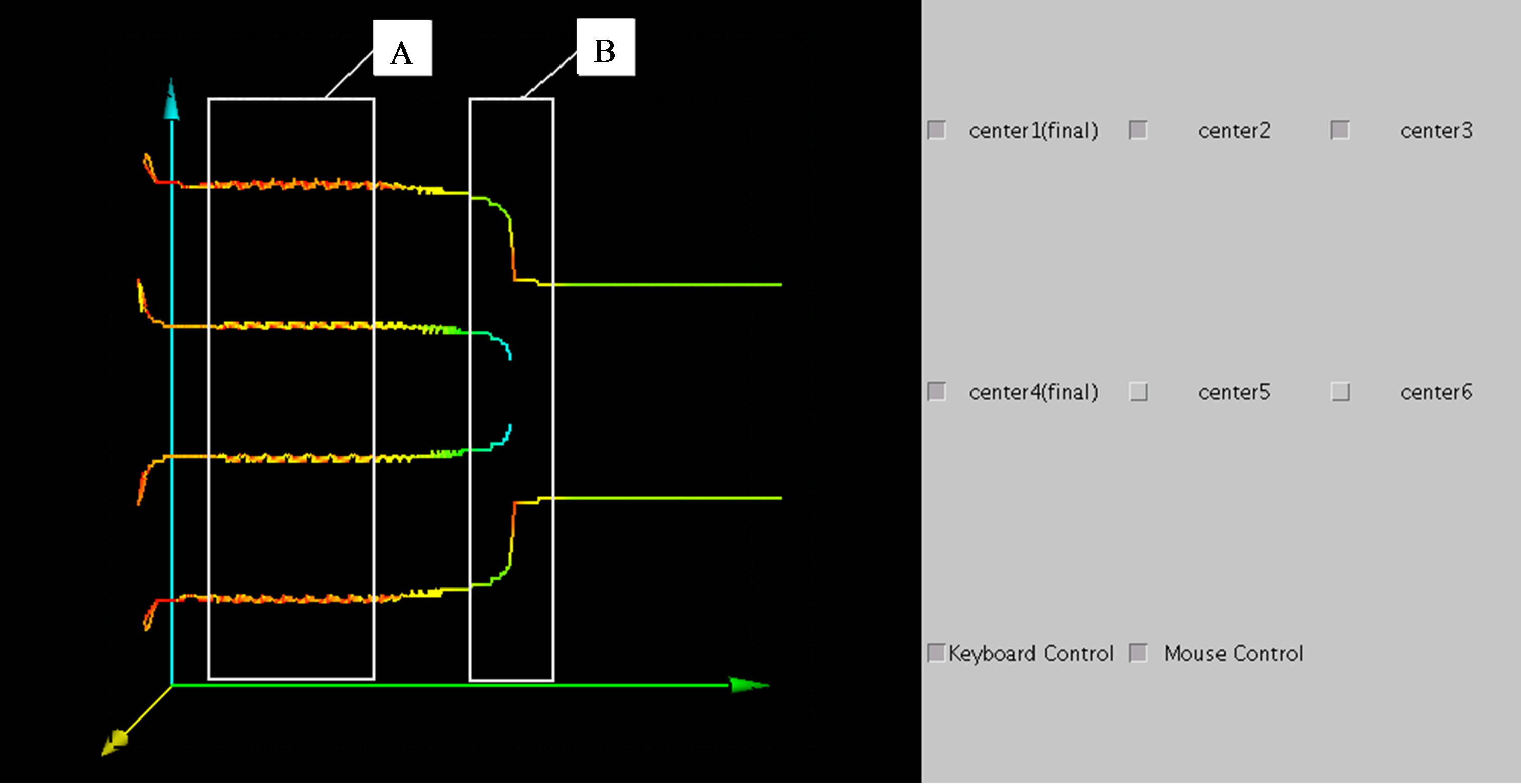 (b)
(b)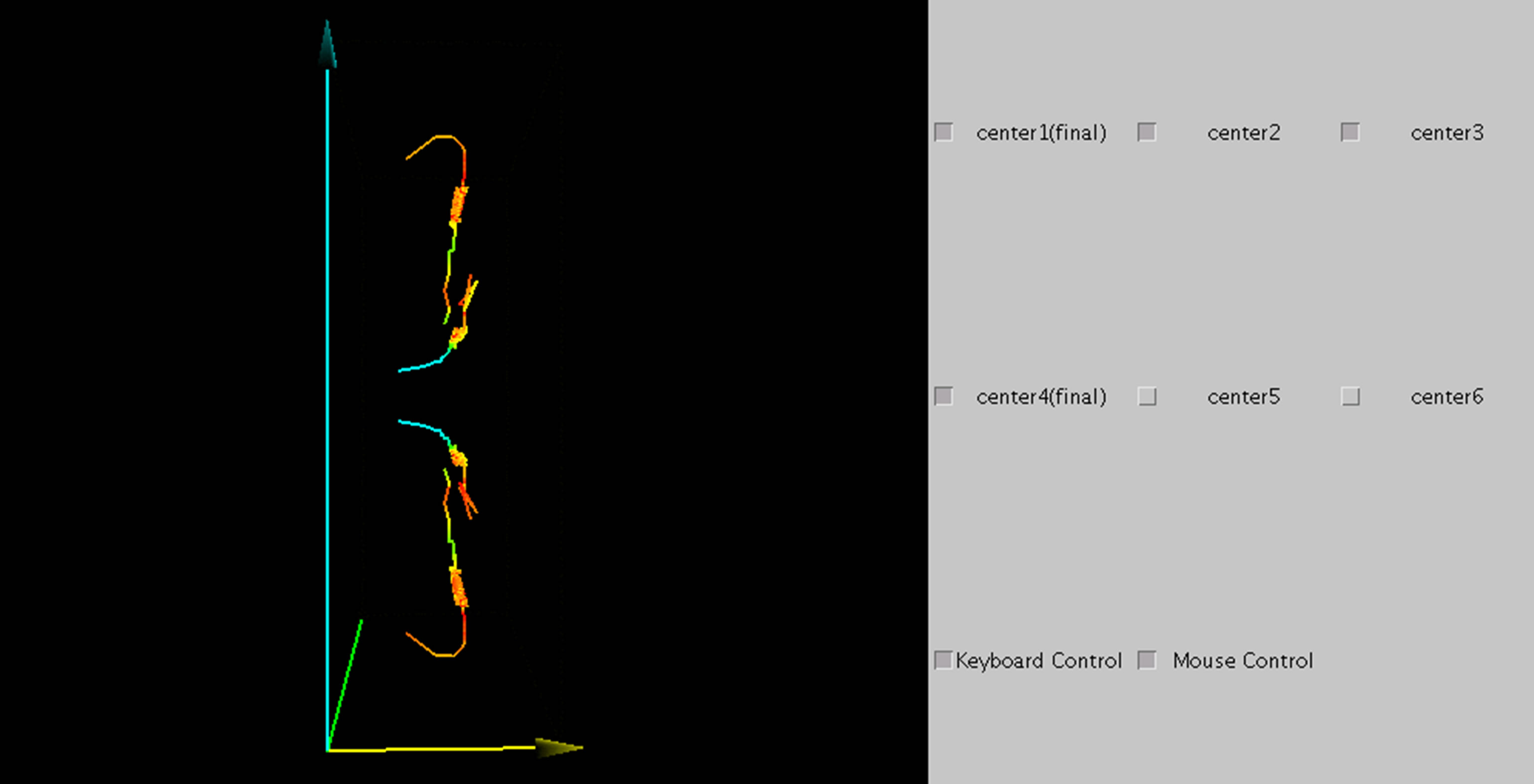 (c)
(c)
Figure 12. Bifurcation process in 3D visualization system. (Re: 700 - 350, Γ: 2.8). (a) 3D visualization system. (Volume-averaged energy); (b) Nondimensional time-z plane; (c) r-z plane.
In the early stage of mode formation, vortices develop on the midplane in the axial direction and at the upper and lower ends of the inner cylinder. During the mode bifurcation, vortices whose volume-averaged energies are weak disappear. After the bifurcation, the volume-averaged energies of the remaining vortices become large for a while. The volume-averaged energies then decreases and the flow becomes stable. The mean energy is closely related to the bifurcation process.
10. Conclusion
The development of Taylor vortex flow generated in finite-length rotating dual cylinders whose upper and lower ends were fixed was studied. The behavior of the vortices in three dimensions are presented by the Java3D library. This visualization system can be used to analyze the fusion and disappearance of vortices. The formation process for each final mode is nonunique, multiple and complicated. Tracks were colored to analyze the changes in the values of physical quantities. Using this method, changes in the values of physical quantities were measured in detail. During the calculation, the Reynolds number was changed to investigate the behavior of the volumeaveraged energy. When vortices disappear, the volumeaveraged energies of the disappearing vortices are lower than those of the other vortices. When mode bifurcation occurs, the volume-averaged energy becomes large for a while, then decreases gradually, and the flow becomes stable.
REFERENCES
- G. I. Taylor, “Stability of a Viscous Liquid Contained between Two Rotating Cylinders,” Philosophical Transactions of the Royal Society A, Vol. 233, No. 605-615, 1923, pp. 289-343. doi:10.1098/rsta.1923.0008
- J. R. Pacheco, J. M. Lopez and F. Marques, “Pinning of Rotating Waves to Defects in Finite Taylor-Couette Flow,” Journal of Fluid Mechanics, Vol. 666, 2011, pp. 254-272. doi:10.1017/S0022112010004131
- D. Martinand, E. Serre, and R. M. Lueptow, “Absolute and Convective Instability of Cylindrical Couette Flow with Axial and Radial Flows,” Physics of Fluids, Vol. 21, No. 10, 2009, Article ID: 104102. doi:10.1063/1.3243976
- H. Furukawa, M. Hanaki and T. Watanabe, “Influence of Initial Flow on Taylor Vortex Flow,” Journal of Fluid Science and Technology, Vol. 3, No. 1, 2008, pp. 129-136. doi:10.1299/jfst.3.129
- H. Furukawa, T. Watanabe, Y. Toya and I. Nakamura, “Flow Pattern Exchange in the Taylor-Couette System with a Very Small Aspect Ratio,” Physical Review E, Vol. 65, No. 3, 2001, pp. 1-7. doi:10.1103/PhysRevE.65.036306